Civil Rights
Movements, leaders, victories and the continuing fight for equality.

Explore the people, places, events, achievements, struggles and stories that shaped our journey.
Movements, leaders, victories and the continuing fight for equality.
Innovation, patents, science, technology and world-changing contributions.
Pioneers, champions, Negro Leagues, records, activism and excellence.
Meet the people whose lives, choices and achievements shaped the journey.
Black towns, communities, institutions and places where history happened.
Moments that changed communities, movements, institutions and the nation.
In August 1908, a white mob attacked Springfield, Illinois’s Black community, destroying homes and businesses and lynching two Black men. National outrage over the violence helped spur the movement that created the NAACP the following year.
MORE →Reflects the personal views, recollections, and perspective of the author, Mike Davis.
This is a personal recollection on the Move fire on May 13, 1985
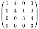
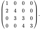
In mathematics, a bidiagonal matrix is a banded matrix with non-zero entries along the main diagonal and either the diagonal above or the diagonal below. This means there are exactly two non-zero diagonals in the matrix.
When the diagonal above the main diagonal has the non-zero entries the matrix is upper bidiagonal. When the diagonal below the main diagonal has the non-zero entries the matrix is lower bidiagonal.
For example, the following matrix is upper bidiagonal:
and the following matrix is lower bidiagonal:
The eigenvalues of a bidiagonal matrix (of either type) are given by the entries of the diagonal.
For a square bidiagonal matrix B, the determinant is simply the product of its diagonal elements:
Additionally, the inverse of a nonsingular upper bidiagonal matrix B is an upper triangular matrix whose entries can be computed explicitly without solving full systems of linear equations.
One variant of the QR algorithm starts with reducing a general matrix into a bidiagonal one,[1] and the singular value decomposition (SVD) uses this method as well.
Reducing a matrix to bidiagonal form is a standard first step in the Golub-Kahan algorithm for computing the SVD. Because Householder reflections or Given rotations can reduce a dense matrix to an equivalent bidiagonal matrix in operations, working with the bidiagonal structure drastically reduces the computational cost of subsequent iterative SVD and QR steps.[2]
For general dense matrices, standard numerical algorithms compute singular values with an absolute error bound proportional to the largest singular value. If the matrix is ill-conditioned, this can result in a total loss of precision for the smallest singular values.[3]
Because of this, specialized algorithms such as the zero-shift bidiagonal QR algorithm or the differential qd (dqd) algorithm developed by James Demmel and William Kahan can compute all the singular values of a bidiagonal matrix to high relative accuracy, regardless of the matrix's condition number.[4]
![[icon]](viewer.php?source=wikipedia&q=File%3AWiki%20letter%20w%20cropped.svg&result=0#selected-result) | This section needs expansion. You can help by adding missing information. (January 2017) |
 | This article about matrices is a stub. You can help Wikipedia by adding missing information. |
 | This computer-programming-related article is a stub. You can help Wikipedia by adding missing information. |
Source: Wikipedia. Article content is retrieved live through the MediaWiki API.
In mathematics, a bidiagonal matrix is a banded matrix with non-zero entries along the main diagonal and either the diagonal above or the diagonal below. This means there are exactly two non-zero diagonals in the matrix. When the diagonal above the main diagonal has the non-zero entries the matrix is upper bidiagonal. When the diagonal below the main diagonal has the non-zero entries the matrix is lower bidiagonal. For example, the following matrix is upper bidiagonal: ( 1 4 0 0 0 4 1 0 0 0 3 4 0 0 0 3 ) {\displaystyle {\begin{pmatrix}1&4&0&0\\0&4&1&0\\0&0&3&4\\0&0&0&3\\\end{pmatrix}}} and the following matrix is lower bidiagonal: ( 1 0 0 0 2 4 0 0 0 3 3 0 0 0 4 3 ) . {\displaystyle {\begin{pmatrix}1&0&0&0\\2&4&0&0\\0&3&3&0\\0&0&4&3\\\end{pmatrix}}.} The eigenvalues of a bidiagonal matrix (of either type) are given by the entries of the diagonal. For a square bidiagonal matrix B, the determinant is simply the product of its diagonal elements: det ( B ) = ∏ i = 1 n b i i {\displaystyle \det(B)=\prod _{i=1}^{n}b_{ii}} Additionally, the inverse of a nonsingular upper bidiagonal matrix B is an upper triangular matrix whose entries can be computed explicitly without solving full systems of linear equations.
Bidiagonalization is one of unitary (orthogonal) matrix decompositions such that U* A V = B, where U and V are unitary (orthogonal) matrices; * denotes Hermitian transpose; and B is upper bidiagonal. A is allowed to be rectangular. For dense matrices, the left and right unitary matrices are obtained by a series of Householder reflections alternately applied from the left and right. This is known as Golub-Kahan bidiagonalization. For large matrices, they are calculated iteratively by using Lanczos method, referred to as Golub-Kahan-Lanczos method. Bidiagonalization has a very similar structure to the singular value decomposition (SVD). However, it is computed within finite operations, while SVD requires iterative schemes to find singular values. The latter is because the squared singular values are the roots of characteristic polynomials of A* A, where A is assumed to be tall.
In linear algebra, a diagonal matrix is a matrix in which the entries outside the main diagonal are all zero; the term usually refers to square matrices. Elements of the main diagonal can either be zero or nonzero. An example of a 2×2 diagonal matrix is [ 3 0 0 2 ] {\displaystyle \left[{\begin{smallmatrix}3&0\\0&2\end{smallmatrix}}\right]} , while an example of a 3×3 diagonal matrix is [ 6 0 0 0 5 0 0 0 4 ] {\displaystyle \left[{\begin{smallmatrix}6&0&0\\0&5&0\\0&0&4\end{smallmatrix}}\right]} . An identity matrix of any size, or any multiple of it is a diagonal matrix called a scalar matrix, for example, [ 0.5 0 0 0.5 ] {\displaystyle \left[{\begin{smallmatrix}0.5&0\\0&0.5\end{smallmatrix}}\right]} . In geometry, a diagonal matrix may be used as a scaling matrix, since matrix multiplication with it results in changing scale (size) and possibly also shape; only a scalar matrix results in uniform change in scale.
In mathematics, a Hermitian matrix (or self-adjoint matrix) is a square matrix with complex-valued entries that is equal to its own conjugate transpose. That is, if the element in the j {\displaystyle j} -th row and k {\displaystyle k} -th column of a Hermitian matrix A {\displaystyle A} is some complex number A j k = x + i y {\displaystyle A_{jk}=x+iy} , then the element in the k {\displaystyle k} -th row and j {\displaystyle j} -th column is its complex conjugate A k j = A j k ¯ = x − i y {\displaystyle A_{kj}={\overline {A_{jk}}}=x-iy} , for every pair of indices j {\displaystyle j} and k {\displaystyle k} . Hermitian matrices can be understood as the complex generalization of symmetric real matrices. Using the notation A T {\displaystyle \textstyle A^{\mathsf {T}}} to mean the transpose of A {\displaystyle A} and an overline to mean the entrywise complex conjugate of a matrix, the Hermitian property is equivalent to the equality A = A T ¯ . {\displaystyle A={\overline {A^{\mathsf {T}}}}.} The conjugate transpose of a matrix is often denoted A H {\displaystyle \textstyle A^{\mathsf {H}}} , in terms of which the Hermitian property can be more concisely expressed as A = A H {\displaystyle \textstyle A=A^{\mathsf {H}}} . Equivalent notations in common use include A H {\displaystyle \textstyle A^{\mathsf {H}}} , A † {\displaystyle \textstyle A^{\dagger }} , and A ∗ {\displaystyle \textstyle A^{*}} , although in quantum mechanics, A ∗ {\displaystyle \textstyle A^{*}} typically means the complex conjugate only, and not the conjugate transpose. Hermitian matrices are named after Charles Hermite, who demonstrated in 1855 that matrices of this form share with symmetric real matrices the property of always having real eigenvalues.
Before the 1921 destruction of Tulsa’s Greenwood District, Black residents had created a remarkable center of business and community life. The district included stores, professional offices, entertainment venues and homes owned by Black citizens. Understanding Greenwood means learning what was built—not only what was burned.
MORE →Shirley Chisholm, elected in 1968.