Civil Rights
Movements, leaders, victories and the continuing fight for equality.

Explore the people, places, events, achievements, struggles and stories that shaped our journey.
Movements, leaders, victories and the continuing fight for equality.
Innovation, patents, science, technology and world-changing contributions.
Pioneers, champions, Negro Leagues, records, activism and excellence.
Meet the people whose lives, choices and achievements shaped the journey.
Black towns, communities, institutions and places where history happened.
Moments that changed communities, movements, institutions and the nation.
Mansa Musa was the ruler of the Mali Empire in West Africa. Details recorded here should be sourced; unknown information is left blank.
MORE →Reflects the personal views, recollections, and perspective of the author, Mike Davis.
This is a personal recollection on the Move fire on May 13, 1985
 | This article needs more citations. (June 2019) |
| Part of a series of articles about |
| Calculus |
|---|
In mathematics, a change of variables is a basic technique used to simplify problems in which the original variables are replaced with functions of other variables. The intent is that when expressed in new variables, the problem may become simpler, or equivalent to a better understood problem.
Change of variables is an operation that is related to substitution. However these are different operations, as can be seen when considering differentiation (chain rule) or integration (integration by substitution).
A very simple example of a useful variable change can be seen in the problem of finding the roots of the sixth-degree polynomial:
Sixth-degree polynomial equations are generally impossible to solve in terms of radicals (see Abel–Ruffini theorem). This particular equation, however, may be written
(this is a simple case of a polynomial decomposition). Thus the equation may be simplified by defining a new variable . Substituting x by into the polynomial gives
which is just a quadratic equation with the two solutions:
The solutions in terms of the original variable are obtained by substituting x3 back in for u, which gives
Then, assuming that one is interested only in real solutions, the solutions of the original equation are
Consider the system of equations
where and are positive integers with . (Source: 1991 AIME)
Solving this normally is not very difficult, but it may get a little tedious. However, we can rewrite the second equation as . Making the substitutions and reduces the system to . Solving this gives and . Back-substituting the first ordered pair gives us , which gives the solution Back-substituting the second ordered pair gives us , which gives no solutions. Hence the solution that solves the system is .
Let , be smooth manifolds and let be a -diffeomorphism between them, that is: is a times continuously differentiable, bijective map from to with times continuously differentiable inverse from to . Here may be any natural number (or zero), (smooth) or (analytic).
The map is called a regular coordinate transformation or regular variable substitution, where regular refers to the -ness of . Usually one will write to indicate the replacement of the variable by the variable by substituting the value of in for every occurrence of .
Some systems can be more easily solved when switching to polar coordinates. Consider for example the equation
This may be a potential energy function for some physical problem. If one does not immediately see a solution, one might try the substitution
Note that if runs outside a -length interval, for example, , the map is no longer bijective. Therefore, should be limited to, for example . Notice how is excluded, for is not bijective in the origin ( can take any value, the point will be mapped to (0, 0)). Then, replacing all occurrences of the original variables by the new expressions prescribed by and using the identity , we get
Now the solutions can be readily found: , so or . Applying the inverse of shows that this is equivalent to while . Indeed, we see that for the function vanishes, except for the origin.
Note that, had we allowed , the origin would also have been a solution, though it is not a solution to the original problem. Here the bijectivity of is crucial. The function is always positive (for ), hence the absolute values.
The chain rule is used to simplify complicated differentiation. For example, consider the problem of calculating the derivative
Let with Then:
Difficult integrals may often be evaluated by changing variables; this is enabled by the substitution rule and is analogous to the use of the chain rule above. Difficult integrals may also be solved by simplifying the integral using a change of variables given by the corresponding Jacobian matrix and determinant.[1] Using the Jacobian determinant and the corresponding change of variable that it gives is the basis of coordinate systems such as polar, cylindrical, and spherical coordinate systems.
The following theorem allows us to relate integrals with respect to Lebesgue measure to an equivalent integral with respect to the pullback measure under a parameterization G.[2] The proof is due to approximations of the Jordan content.
Suppose that is an open subset of and is a diffeomorphism.
- If is a Lebesgue measurable function on , then is Lebesgue measurable on . If or then .
- If and is Lebesgue measurable, then is Lebesgue measurable, then .
As a corollary of this theorem, we may compute the Radon–Nikodym derivatives of both the pullback and pushforward measures of under .
The pullback measure in terms of a transformation is defined as . The change of variables formula for pullback measures is
.
Pushforward measure and transformation formula
The pushforward measure in terms of a transformation , is defined as . The change of variables formula for pushforward measures is
.
As a corollary of the change of variables formula for Lebesgue measure, we have that
From which we may obtain
Variable changes for differentiation and integration are taught in elementary calculus and the steps are rarely carried out in full.
The very broad use of variable changes is apparent when considering differential equations, where the independent variables may be changed using the chain rule or the dependent variables are changed resulting in some differentiation to be carried out. Exotic changes, such as the mingling of dependent and independent variables in point and contact transformations, can be very complicated but allow much freedom.
Very often, a general form for a change is substituted into a problem and parameters picked along the way to best simplify the problem.
Probably the simplest change is the scaling and shifting of variables, that is replacing them with new variables that are "stretched" and "moved" by constant amounts. This is very common in practical applications to get physical parameters out of problems. For an nth order derivative, the change simply results in
where
This may be shown readily through the chain rule and linearity of differentiation. This change is very common in practical applications to get physical parameters out of problems, for example, the boundary value problem
describes parallel fluid flow between flat solid walls separated by a distance δ; μ is the viscosity and the pressure gradient, both constants. By scaling the variables the problem becomes
where
Scaling is useful for many reasons. It simplifies analysis both by reducing the number of parameters and by simply making the problem neater. Proper scaling may normalize variables, that is make them have a sensible unitless range such as 0 to 1. Finally, if a problem mandates numeric solution, the fewer the parameters the smaller the number of computations.
Consider a system of equations
for a given function . The mass can be eliminated by the (trivial) substitution . Clearly this is a bijective map from to . Under the substitution the system becomes
Given a force field , Newton's equations of motion are
Lagrange examined how these equations of motion change under an arbitrary substitution of variables ,
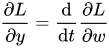
He found that the equations
are equivalent to Newton's equations for the function , where T is the kinetic, and V the potential energy.
In fact, when the substitution is chosen well (exploiting for example symmetries and constraints of the system) these equations are much easier to solve than Newton's equations in Cartesian coordinates.
Source: Wikipedia. Article content is retrieved live through the MediaWiki API.
In mathematics, a change of variables is a basic technique used to simplify problems in which the original variables are replaced with functions of other variables. The intent is that when expressed in new variables, the problem may become simpler, or equivalent to a better understood problem. Change of variables is an operation that is related to substitution. However these are different operations, as can be seen when considering differentiation (chain rule) or integration (integration by substitution). A very simple example of a useful variable change can be seen in the problem of finding the roots of the sixth-degree polynomial: x 6 − 9 x 3 + 8 = 0. {\displaystyle x^{6}-9x^{3}+8=0.} Sixth-degree polynomial equations are generally impossible to solve in terms of radicals (see Abel–Ruffini theorem). This particular equation, however, may be written ( x 3 ) 2 − 9 ( x 3 ) + 8 = 0 {\displaystyle (x^{3})^{2}-9(x^{3})+8=0} (this is a simple case of a polynomial decomposition). Thus the equation may be simplified by defining a new variable u = x 3 {\displaystyle u=x^{3}} . Substituting x by u 3 {\displaystyle {\sqrt[{3}]{u}}} into the polynomial gives u 2 − 9 u + 8 = 0 , {\displaystyle u^{2}-9u+8=0,} which is just a quadratic equation with the two solutions: u = 1 and u = 8. {\displaystyle u=1\quad {\text{and}}\quad u=8.} The solutions in terms of the original variable are obtained by substituting x3 back in for u, which gives x 3 = 1 and x 3 = 8. {\displaystyle x^{3}=1\quad {\text{and}}\quad x^{3}=8.} Then, assuming that one is interested only in real solutions, the solutions of the original equation are x = ( 1 ) 1 / 3 = 1 and x = ( 8 ) 1 / 3 = 2. {\displaystyle x=(1)^{1/3}=1\quad {\text{and}}\quad x=(8)^{1/3}=2.}
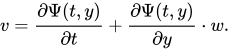
Often a partial differential equation can be reduced to a simpler form with a known solution by a suitable change of variables. The article discusses change of variable for PDEs below in two ways: by example; by giving the theory of the method.
A differential equation can be homogeneous in either of two respects. A first order differential equation is said to be homogeneous if it may be written f ( x , y ) d y = g ( x , y ) d x , {\displaystyle f(x,y)\,dy=g(x,y)\,dx,} where f and g are homogeneous functions of the same degree of x and y. In this case, the change of variable y = ux leads to an equation of the form d x x = h ( u ) d u , {\displaystyle {\frac {dx}{x}}=h(u)\,du,} which is easy to solve by integration of the two members. Otherwise, a differential equation is homogeneous if it is a homogeneous function of the unknown function and its derivatives. In the case of linear differential equations, this means that there are no constant terms. The solutions of any linear ordinary differential equation of any order may be deduced by integration from the solution of the homogeneous equation obtained by removing the constant term.
In statistical mechanics, the Lee–Yang theorem states that if partition functions of certain models in statistical field theory with ferromagnetic interactions are considered as functions of an external field, then all zeros are purely imaginary (or on the unit circle after a change of variable). The first version was proved for the Ising model by T. D. Lee and C. N. Yang (1952) (Lee & Yang 1952). Their result was later extended to more general models by several people. Asano in 1970 extended the Lee–Yang theorem to the Heisenberg model and provided a simpler proof using Asano contractions. Simon & Griffiths (1973) extended the Lee–Yang theorem to certain continuous probability distributions by approximating them by a superposition of Ising models. Newman (1974) gave a general theorem stating roughly that the Lee–Yang theorem holds for a ferromagnetic interaction provided it holds for zero interaction. Lieb & Sokal (1981) generalized Newman's result from measures on R to measures on higher-dimensional Euclidean space. There has been some speculation about a relationship between the Lee–Yang theorem and the Riemann hypothesis about the Riemann zeta function; see (Knauf 1999).
Before the 1921 destruction of Tulsa’s Greenwood District, Black residents had created a remarkable center of business and community life. The district included stores, professional offices, entertainment venues and homes owned by Black citizens. Understanding Greenwood means learning what was built—not only what was burned.
MORE →Mae Jemison, aboard Space Shuttle Endeavour in 1992.





![{\displaystyle (0,\infty ]\times [0,2\pi )}](https://wikimedia.org/api/rest_v1/media/math/render/svg/1418570ad43959fec6dcd6c3e52c9e5b0ccf81ee)