Explore Black History

Competitive equilibrium (also called: Walrasian equilibrium) is a concept of economic equilibrium, introduced by Kenneth Arrow and Gérard Debreu in 1951,^[1] appropriate for the analysis of commodity markets with flexible prices and many traders, and serving as the benchmark of efficiency in economic analysis. It relies crucially on the assumption of a competitive environment where each trader decides upon a quantity that is so small compared to the total quantity traded in the market that their individual transactions have no influence on the prices. Competitive markets are an ideal standard by which other market structures are evaluated.

A competitive equilibrium (CE) consists of two elements:

• A price function ${\displaystyle P}$. It takes as argument a vector representing a bundle of commodities, and returns a positive real number that represents its price. Usually the price function is linear - it is represented as a vector of prices, a price for each commodity type.
• An allocation matrix ${\displaystyle X}$. For every ${\displaystyle i\in 1,\dots ,n}$, ${\displaystyle X_{i}}$ is the vector of commodities allotted to agent ${\displaystyle i}$.

These elements should satisfy the following requirement:

• Satisfaction (market-envy-freeness): Every agent weakly prefers his bundle to any other affordable bundle:

${\displaystyle \forall i\in 1,\dots ,n}$, if ${\displaystyle P(Y)\leq P(X_{i})}$ then ${\displaystyle Y\preceq _{i}X_{i}}$.

Often, there is an initial endowment matrix ${\displaystyle E}$: for every ${\displaystyle i\in 1,\dots ,n}$, ${\displaystyle E_{i}}$ is the initial endowment of agent ${\displaystyle i}$. Then, a CE should satisfy some additional requirements:

• Market Clearance: the demand equals the supply, no items are created or destroyed:

${\displaystyle \sum _{i=1}^{n}X_{i}=\sum _{i=1}^{n}E_{i}}$.

• Individual Rationality: all agents are better-off after the trade than before the trade:

${\displaystyle \forall i\in 1,\dots ,n:X_{i}\succeq _{i}E_{i}}$.

• Budget Balance: all agents can afford their allocation given their endowment:

${\displaystyle \forall i\in 1,\dots ,n:P(X_{i})\leq P(E_{i})}$.

This definition explicitly allows for the possibility that there may be multiple commodity arrays that are equally appealing. Also for zero prices. An alternative definition^[2] relies on the concept of a demand-set. Given a price function P and an agent with a utility function U, a certain bundle of goods x is in the demand-set of the agent if: ${\displaystyle U(x)-P(x)\geq U(y)-P(y)}$ for every other bundle y. A competitive equilibrium is a price function P and an allocation matrix X such that:

• The bundle allocated by X to each agent is in that agent's demand-set for the price-vector P;
• Every good which has a positive price is fully allocated (i.e. every unallocated item has price 0).

In some cases it is useful to define an equilibrium in which the rationality condition is relaxed.^[3] Given a positive value ${\displaystyle \epsilon }$ (measured in monetary units, e.g., dollars), a price vector ${\displaystyle P}$ and a bundle ${\displaystyle x}$, define ${\displaystyle P_{\epsilon }^{x}}$ as a price vector in which all items in x have the same price they have in P, and all items not in x are priced ${\displaystyle \epsilon }$ more than their price in P.

In a ${\displaystyle \epsilon }$-competitive-equilibrium, the bundle x allocated to an agent should be in that agent's demand-set for the modified price vector, ${\displaystyle P_{\epsilon }^{x}}$.

This approximation is realistic when there are buy/sell commissions. For example, suppose that an agent has to pay ${\displaystyle \epsilon }$ dollars for buying a unit of an item, in addition to that item's price. That agent will keep his current bundle as long as it is in the demand-set for price vector ${\displaystyle P_{\epsilon }^{x}}$. This makes the equilibrium more stable.

The following examples involve an exchange economy with two agents, Jane and Kelvin, two goods e.g. bananas (x) and apples (y), and no money.

1. Graphical example: Suppose that the initial allocation is at point X, where Jane has more apples than Kelvin does and Kelvin has more bananas than Jane does.

By looking at their indifference curves ${\displaystyle J_{1}}$ of Jane and ${\displaystyle K_{1}}$ of Kelvin, we can see that this is not an equilibrium - both agents are willing to trade with each other at the prices ${\displaystyle P_{x}}$ and ${\displaystyle P_{y}}$. After trading, both Jane and Kelvin move to an indifference curve which depicts a higher level of utility, ${\displaystyle J_{2}}$ and ${\displaystyle K_{2}}$. The new indifference curves intersect at point E. The slope of the tangent of both curves equals -${\displaystyle P_{x}/P_{y}}$.

And the ${\displaystyle MRS_{Jane}=P_{x}/P_{y}}$; ${\displaystyle MRS_{Kelvin}=P_{x}/P_{y}}$. The marginal rate of substitution (MRS) of Jane equals that of Kelvin. Therefore, the 2 individuals society reaches Pareto efficiency, where there is no way to make Jane or Kelvin better off without making the other worse off.

2. Arithmetic example:^{[4]: 322–323} suppose that both agents have Cobb–Douglas utilities:

${\displaystyle u_{J}(x,y)=x^{a}y^{1-a}}$

${\displaystyle u_{K}(x,y)=x^{b}y^{1-b}}$

where ${\displaystyle a,b}$ are constants.

Suppose the initial endowment is ${\displaystyle E=[(1,0),(0,1)]}$.

The demand function of Jane for x is:

${\displaystyle x_{J}(p_{x},p_{y},I_{J})={\frac {a\cdot I_{J}}{p_{x}}}={\frac {a\cdot (1\cdot p_{x})}{p_{x}}}=a}$

The demand function of Kelvin for x is:

${\displaystyle x_{K}(p_{x},p_{y},I_{K})={\frac {b\cdot I_{K}}{p_{x}}}={\frac {b\cdot p_{y}}{p_{x}}}}$

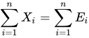
The market clearance condition for x is:

${\displaystyle x_{J}+x_{K}=E_{J,x}+E_{K,x}=1}$

This equation yields the equilibrium price ratio:

${\displaystyle {\frac {p_{y}}{p_{x}}}={\frac {1-a}{b}}}$

We could do a similar calculation for y, but this is not needed, since Walras' law guarantees that the results will be the same. Note that in CE, only relative prices are determined; we can normalize the prices, e.g., by requiring that ${\displaystyle p_{x}+p_{y}=1}$. Then we get ${\displaystyle p_{x}={\frac {b}{1+b-a}},p_{y}={\frac {1-a}{1+b-a}}}$. But any other normalization will also work.

3. Non-existence example: Suppose the agents' utilities are:

${\displaystyle u_{J}(x,y)=u_{K}(x,y)=\max(x,y)}$

and the initial endowment is [(2,1),(2,1)]. In CE, every agent must have either only x or only y (the other product does not contribute anything to the utility so the agent would like to exchange it away). Hence, the only possible CE allocations are [(4,0),(0,2)] and [(0,2),(4,0)]. Since the agents have the same income, necessarily ${\displaystyle p_{y}=2p_{x}}$. But then, the agent holding 2 units of y will want to exchange them for 4 units of x.

4. For existence and non-existence examples involving linear utilities, see Linear utility#Examples.

When there are indivisible items in the economy, it is common to assume that there is also money, which is divisible. The agents have quasilinear utility functions: their utility is the amount of money they have plus the utility from the bundle of items they hold.

A. Single item: Alice has a car which she values as 10. Bob has no car, and he values Alice's car as 20. A possible CE is: the price of the car is 15, Bob gets the car and pays 15 to Alice. This is an equilibrium because the market is cleared and both agents prefer their final bundle to their initial bundle. In fact, every price between 10 and 20 will be a CE price, with the same allocation. The same situation holds when the car is not initially held by Alice but rather in an auction in which both Alice and Bob are buyers: the car will go to Bob and the price will be anywhere between 10 and 20.

On the other hand, any price below 10 is not an equilibrium price because there is an excess demand (both Alice and Bob want the car at that price), and any price above 20 is not an equilibrium price because there is an excess supply (neither Alice nor Bob want the car at that price).

This example is a special case of a double auction.

B. Substitutes: A car and a horse are sold in an auction. Alice only cares about transportation, so for her these are perfect substitutes: she gets utility 8 from the horse, 9 from the car, and if she has both of them then she uses only the car so her utility is 9. Bob gets a utility of 5 from the horse and 7 from the car, but if he has both of them then his utility is 11 since he also likes the horse as a pet. In this case it is more difficult to find an equilibrium (see below). A possible equilibrium is that Alice buys the horse for 5 and Bob buys the car for 7. This is an equilibrium since Bob wouldn't like to pay 5 for the horse which will give him only 4 additional utility, and Alice wouldn't like to pay 7 for the car which will give her only 1 additional utility.

C. Complements:^[5] A horse and a carriage are sold in an auction. There are two potential buyers: AND and XOR. AND wants only the horse and the carriage together - they receive a utility of ${\displaystyle v_{and}}$ from holding both of them but a utility of 0 for holding only one of them. XOR wants either the horse or the carriage but doesn't need both - they receive a utility of ${\displaystyle v_{xor}}$ from holding one of them and the same utility for holding both of them. Here, when ${\displaystyle v_{and}<2v_{xor}}$, a competitive equilibrium does not exist, i.e., no price will clear the market. Proof: consider the following options for the sum of the prices (horse-price + carriage-price):

• The sum is less than ${\displaystyle v_{and}}$. Then, AND wants both items. Since the price of at least one item is less than ${\displaystyle v_{xor}}$, XOR wants that item, so there is excess demand.
• The sum is exactly ${\displaystyle v_{and}}$. Then, AND is indifferent between buying both items and not buying any item. But XOR still wants exactly one item, so there is either excess demand or excess supply.
• The sum is more than ${\displaystyle v_{and}}$. Then, AND wants no item and XOR still wants at most a single item, so there is excess supply.

D. Unit-demand consumers: There are n consumers. Each consumer has an index ${\displaystyle i=1,...,n}$. There is a single type of good. Each consumer ${\displaystyle i}$ wants at most a single unit of the good, which gives him a utility of ${\displaystyle u(i)}$. The consumers are ordered such that ${\displaystyle u}$ is a weakly increasing function of ${\displaystyle i}$. If the supply is ${\displaystyle k\leq n}$ units, then any price ${\displaystyle p}$ satisfying ${\displaystyle u(n-k)\leq p\leq u(n-k+1)}$ is an equilibrium price, since there are k consumers that either want to buy the product or indifferent between buying and not buying it. Note that an increase in supply causes a decrease in price.

The Arrow–Debreu model shows that a CE exists in every exchange economy with divisible goods satisfying the following conditions:

• All agents have strictly convex preferences;
• All goods are desirable. This means that, if any good ${\displaystyle j}$ is given for free (${\displaystyle p_{j}=0}$), then all agents want as much as possible from that good.

The proof proceeds in several steps.^{[4]: 319–322}

A. For concreteness, assume that there are ${\displaystyle n}$ agents and ${\displaystyle k}$ divisible goods. Normalize the prices such that their sum is 1, i.e. ${\displaystyle \sum _{j=1}^{k}p_{j}=1}$. Then the space of all possible prices is the ${\displaystyle k-1}$-dimensional unit simplex in ${\displaystyle \mathbb {R} ^{k}}$. We call this simplex the price simplex.

B. Let ${\displaystyle z}$ be the excess demand function. This is a function of the price vector ${\displaystyle p}$ when the initial endowment ${\displaystyle E}$ is kept constant:

${\displaystyle z(p)=\sum _{i=1}^{n}\left({x_{i}(p,p\cdot E_{i})-E_{i}}\right)}$

It is known that, when the agents have strictly convex preferences, the Marshallian demand function is continuous. Hence, ${\displaystyle z}$ is also a continuous function of ${\displaystyle p}$.

C. Define the following function from the price simplex to itself:

${\displaystyle g_{i}(p)={\frac {p_{i}+\max(0,z_{i}(p))}{1+\sum _{j=1}^{k}\max(0,z_{j}(p))}},\forall i\in 1,\dots ,k}$

This is a continuous function, so by the Brouwer fixed-point theorem there is a price vector ${\displaystyle p^{*}}$ such that:

${\displaystyle p^{*}=g(p^{*})}$

so,

${\displaystyle p_{i}^{*}={\frac {p_{i}+\max(0,z_{i}(p))}{1+\sum _{j=1}^{k}\max(0,z_{j}(p))}},\forall i\in 1,\dots ,k}$

D. Using Walras' law and some algebra, it is possible to show that for this price vector, there is no excess demand in any product, i.e:

${\displaystyle z_{j}(p^{*})\leq 0,\forall j\in 1,\dots ,k}$

E. The desirability assumption implies that all products have strictly positive prices:

${\displaystyle p_{j}>0,\forall j\in 1,\dots ,k}$

By Walras' law, ${\displaystyle p^{*}\cdot z(p^{*})=0}$. But this implies that the inequality above must be an equality:

${\displaystyle z_{j}(p^{*})=0,\forall j\in 1,\dots ,k}$

This means that ${\displaystyle p^{*}}$ is a price vector of a competitive equilibrium.

Note that Linear utilities are only weakly convex, so they do not qualify for the Arrow–Debreu model. However, David Gale proved that a CE exists in every linear exchange economy satisfying certain conditions. For details see Linear utilities#Existence of competitive equilibrium.

Algorithms for computing the market equilibrium are described in market equilibrium computation.

In the examples above, a competitive equilibrium existed when the items were substitutes but not when the items were complements. This is not a coincidence.

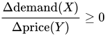
Given a utility function on two goods X and Y, say that the goods are weakly gross-substitute (GS) if they are either independent goods or gross substitute goods, but not complementary goods. This means that ${\displaystyle {\frac {\Delta {\text{demand}}(X)}{\Delta {\text{price}}(Y)}}\geq 0}$. I.e., if the price of Y increases, then the demand for X either remains constant or increases, but does not decrease. If the price of Y decreases, then the demand for X either remains constant or decreases.

A utility function is called GS if, according to this utility function, all pairs of different goods are GS. With a GS utility function, if an agent has a demand set at a given price vector, and the prices of some items increase, then the agent has a demand set which includes all the items whose price remained constant.^[3][6] He may decide that he doesn't want an item which has become more expensive; he may also decide that he wants another item instead (a substitute); but he may not decide that he doesn't want a third item whose price hasn't changed.

When the utility functions of all agents are GS, a competitive equilibrium always exists.^[7]

Moreover, the set of GS valuations is the largest set containing unit demand valuations for which the existence of competitive equilibrium is guaranteed: for any non-GS valuation, there exist unit-demand valuations such that a competitive equilibrium does not exist for these unit-demand valuations coupled with the given non-GS valuation.^[8]

For the computational problem of finding a competitive equilibrium in a special kind of a market, see Fisher market#indivisible.

By the fundamental theorems of welfare economics, any CE allocation is Pareto efficient, and any efficient allocation can be sustainable by a competitive equilibrium. Furthermore, by Varian's theorems, a CE allocation in which all agents have the same income is also envy-free.

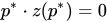
At the competitive equilibrium, the value society places on a good is equivalent to the value of the resources given up to produce it (marginal benefit equals marginal cost). This ensures allocative efficiency: the additional value society places on another unit of the good is equal to what society must give up in resources to produce it.^[9]

Note that microeconomic analysis does not assume additive utility, nor does it assume any interpersonal utility tradeoffs. Efficiency, therefore, refers to the absence of Pareto improvements. It does not in any way opine on the fairness of the allocation (in the sense of distributive justice or equity). An efficient equilibrium could be one where one player has all the goods and other players have none (in an extreme example), which is efficient in the sense that one may not be able to find a Pareto improvement - which makes all players (including the one with everything in this case) better off (for a strict Pareto improvement), or not worse off.

In the case of indivisible items, we have the following strong versions of the two welfare theorems:^[2]

1. Any competitive equilibrium maximizes the social welfare (the sum of utilities), not only over all realistic assignments of items, but also over all fractional assignments of items. I.e., even if we could assign fractions of an item to different people, we couldn't do better than a competitive equilibrium in which only whole items are assigned.
2. If there is an integral assignment (with no fractional assignments) that maximizes the social welfare, then there is a competitive equilibrium with that assignment.

In the case of indivisible item assignment, when the utility functions of all agents are GS (and thus an equilibrium exists), it is possible to find a competitive equilibrium using an ascending auction. In an ascending auction, the auctioneer publishes a price vector, initially zero, and the buyers declare their favorite bundle under these prices. In case each item is desired by at most a single bidder, the items are divided and the auction is over. In case there is an excess demand on one or more items, the auctioneer increases the price of an over-demanded item by a small amount (e.g. a dollar), and the buyers bid again.

Several different ascending-auction mechanisms have been suggested in the literature.^[3][7][10] Such mechanisms are often called Walrasian auction, Walrasian tâtonnement or English auction.

• Envy-free pricing - a relaxation of Walrasian equilibrium in which some items may remain unallocated.
• Fisher market - a simplified market model, with a single seller and many buyers, in which a CE can be computed efficiently.
• Allocative efficiency
• Economic equilibrium
• General equilibrium theory
• Walrasian auction

• Richter, M. K.; Wong, K. C. (1999). "Non-computability of competitive equilibrium". Economic Theory. 14: 1–27. doi:10.1007/s001990050281. S2CID 121248813.

• Competitive equilibrium, Walrasian equilibrium and Walrasian auction in Economics Stack Exchange.