Explore Black History

In frequentist inference, a confidence interval (CI) determines lower and upper bounds likely to contain (in repeated sampling) the true value of an unknown statistical parameter, such as a population mean.^[1] Rather than reporting a single point estimate (e.g. "the average screen time is 3 hours per day"), a confidence interval provides an interval, such as from 2 hours to 4 hours.

A confidence interval is based on a pre-defined coverage probability, called confidence level, typically 95%. A 95% confidence level does not imply a 95% probability that the true parameter lies within a particular CI calculated from a sample (such interpretation would be associated with the credible interval in Bayesian inference). The confidence level instead reflects the long-run performance of the method used to generate the interval.^[2][3] In other words, if the same sampling procedure were repeated 100 times from the same population, approximately 95 of the resulting intervals would be expected to contain the true population mean. The frequentist approach sees the true population mean as a fixed unknown constant, while the confidence interval is calculated using data from a random sample. Because the sample is random, the interval endpoints are random variables.

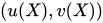
Let ${\displaystyle X}$ be a random sample from a probability distribution with statistical parameter ${\displaystyle (\theta ,\varphi )}$. Here, ${\displaystyle \theta }$ is the quantity to be estimated, while ${\displaystyle \varphi }$ includes other parameters (if any) that determine the distribution. A confidence interval for the parameter ${\displaystyle \theta }$, with confidence level or coefficient ${\displaystyle \gamma }$, is an interval ${\displaystyle (u(X),v(X))}$ determined by random variables ${\displaystyle u(X)}$ and ${\displaystyle v(X)}$ with the property: $${\displaystyle P(u(X)<\theta <v(X))=\gamma \quad {\text{for all }}(\theta ,\varphi ).}$$

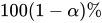
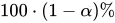
The number ${\displaystyle \gamma }$, which is typically large (e.g. 0.95), is sometimes given in the form ${\displaystyle 1-\alpha }$ (or as a percentage ${\displaystyle 100\cdot (1-\alpha )\%}$), where ${\displaystyle \alpha }$ is a small positive number, often 0.05. It means that the interval ${\textstyle (u(X),v(X))}$ has a probability ${\textstyle \gamma }$ of covering the value of ${\textstyle \theta }$ in repeated sampling.

Alternatively, some authors^[4] simply require that

$${\displaystyle P(u(X)<\theta <v(X))\geq \ \gamma \quad {\text{for all }}(\theta ,\varphi ).}$$ The confidence level can be described as "at least ${\displaystyle 100\gamma \%}$". When it is known that the coverage probability can be strictly larger than ${\displaystyle \gamma }$ for some parameter values, the confidence interval is called conservative, i.e., it errs on the safe side.

In many applications, confidence intervals that have exactly the required confidence level are hard to construct, but approximate intervals can be computed. The rule for constructing the interval may be accepted if

$${\displaystyle P(u(X)<\theta <v(X))\approx \ \gamma }$$

to an acceptable level of approximation.

There are many ways of calculating confidence intervals, and the best method depends on the situation. Two widely applicable methods are bootstrapping and the central limit theorem.^[2] The latter method works only if the sample is large, since it entails calculating the sample mean ${\displaystyle {\bar {X}}}$ and sample standard deviation ${\displaystyle S}$ and using the asymptotically standard normal quantity

$${\displaystyle {\frac {{\bar {X}}-\mu }{S/{\sqrt {n}}}}}$$

where ${\textstyle \mu }$ and ${\displaystyle n}$ are the population mean and the sample size, respectively.

Suppose ${\displaystyle X_{1},\ldots ,X_{n}}$ is an independent sample from a normally distributed population with unknown parameters mean ${\displaystyle \mu }$ and variance ${\displaystyle \sigma ^{2}.}$ Define the sample mean ${\displaystyle {\bar {X}}}$ and unbiased sample variance ${\displaystyle S^{2}}$ as

$${\displaystyle {\begin{aligned}{\bar {X}}&={\frac {1}{n}}\left(X_{1}+\cdots +X_{n}\right),\\S^{2}&={\frac {1}{n-1}}\sum _{i=1}^{n}\left(X_{i}-{\bar {X}}\right)^{2}.\end{aligned}}}$$

Then the value

$${\displaystyle T={\frac {{\bar {X}}-\mu }{S/{\sqrt {n}}}}}$$

has a Student's t distribution with ${\textstyle n-1}$ degrees of freedom.^[5] This value is useful because its distribution does not depend on the values of the unobservable parameters ${\textstyle \mu }$ and ${\textstyle \sigma ^{2}}$; i.e., it is a pivotal quantity.

Suppose we wanted to calculate a 95% confidence interval for ${\textstyle \mu .}$ First, let ${\textstyle c}$ be the 97.5th percentile of the distribution of ${\textstyle T}$. Then there is a 2.5% chance that ${\textstyle T}$ will be less than ${\textstyle -c}$ and a 2.5% chance that it will be larger than ${\textstyle +c}$ (as the t distribution is symmetric about 0). In other words,

$${\displaystyle P_{T}(-c\leq T\leq c)=0.95.}$$

Consequently, by replacing ${\textstyle T}$ with ${\displaystyle {\frac {{\bar {X}}-\mu }{S/{\sqrt {n}}}}}$ and re-arranging terms,

$${\displaystyle P_{X}{\left({\bar {X}}-{\frac {cS}{\sqrt {n}}}\leq \mu \leq {\bar {X}}+{\frac {cS}{\sqrt {n}}}\right)}=0.95}$$

where ${\displaystyle P_{X}}$ is the probability measure for the sample ${\displaystyle X_{1},\ldots ,X_{n}}$.

It means that there is 95% probability with which this condition ${\displaystyle {\bar {X}}-{\frac {cS}{\sqrt {n}}}\leq \mu \leq {\bar {X}}+{\frac {cS}{\sqrt {n}}}}$ occurs in repeated sampling. After observing a sample, we find values ${\displaystyle {\bar {x}}}$ for ${\displaystyle {\bar {X}}}$ and ${\displaystyle s}$ for ${\displaystyle S,}$ from which we compute the below interval, and we say it is a 95% confidence interval for the mean.

$${\displaystyle \left[{\bar {x}}-{\frac {cs}{\sqrt {n}}},{\bar {x}}+{\frac {cs}{\sqrt {n}}}\right].}$$

Various interpretations of a confidence interval can be given (taking the 95% confidence interval as an example in the following).

• The confidence interval can be expressed in terms of a long-run frequency in repeated samples (or in resampling): "Were this procedure to be repeated on numerous samples, the proportion of calculated 95% confidence intervals that encompassed the true value of the population parameter would tend toward 95%."^[6]
• The confidence interval can be expressed in terms of probability with respect to a single theoretical (yet to be realized) sample: "There is a 95% probability that the 95% confidence interval calculated from a given future sample will cover the true value of the population parameter."^[7] This essentially reframes the "repeated samples" interpretation as a probability rather than a frequency.
• The confidence interval can be expressed in terms of statistical significance, e.g.: "The 95% confidence interval represents values that are not statistically significantly different from the point estimate at the .05 level."^[8]

Confidence intervals and levels are frequently misunderstood, and published studies have shown that even professional scientists often misinterpret them.^[9]

Contrary to common misconceptions, a 95% confidence level does not mean that:

• for a given realized interval there is a 95% probability that the population parameter lies within the interval;^[10][11]
• 95% of the sample data lie within the confidence interval;^[1] or
• there is a 95% probability of the parameter estimate from a repeat of the experiment falling within the confidence interval computed from a given experiment.^[11]

For example, suppose a factory produces metal rods, and a random sample of 25 rods gives a 95% confidence interval of 36.8 to 39.0 mm for the population mean length.^[12]

• It is incorrect to say that there is a 95% probability that the true population mean lies within this interval: the true mean is fixed, not random. The true mean could be 37 mm, which is within the confidence interval, or 40 mm, which is not; in any case, whether it falls between 36.8 and 39.0 mm is a matter of fact, not probability.
• It is not necessarily true that the lengths of 95% of the sampled rods lie within this interval. In this case, it cannot be true: 95% of 25 is not an integer.
• It is not generally true that there is a 95% probability that the sample mean length (an estimate of the population mean length) in a second sample would fall within this interval. In fact, if the true mean length is far from this specific confidence interval, it could be very unlikely that the next sample mean falls within the interval.

Instead, the 95% confidence level means that if we took 100 such samples, we would expect the true population mean to lie within approximately 95 of the calculated intervals.^{[1][10][11][12]}

Interpreting confidence intervals is especially tricky when multiple groups are involved. Two common misconceptions are: that two groups are significantly different if their CIs "just touch," and that they differ when one group's CI excludes the other's mean. Neither of these is true in general, but even experienced researchers often make these mistakes.^[13]

A confidence interval is used to estimate a population parameter, such as the mean. For example, the expected value of a fair six-sided die is 3.5. Based on repeated sampling, after computing many 95% confidence intervals, roughly 95% of them will contain 3.5 (and the width of the confidence interval shrinks with sample size).

A prediction interval, on the other hand, provides a range within which a future individual observation is expected to fall with a certain probability. In the case of a single roll of a fair six-sided die, an exact 95% prediction interval does not exist. However, there are exact 95% prediction intervals for rolling a twenty-sided die. One such interval is ${\displaystyle [1,19]}$, since 95% of the time the roll will result in a 19 or less, and the remaining 5% will result in a 20.

The key distinction is that confidence intervals quantify uncertainty in estimating parameters, while prediction intervals quantify uncertainty in forecasting future observations.

In many common settings, such as estimating the mean of a normal distribution with known variance,^[14] confidence intervals coincide with credible intervals under non-informative priors. In such cases, common misconceptions about confidence intervals (e.g. interpreting them as probability statements about the parameter) may yield practically correct conclusions.

Welch^[15] presented an example which clearly shows the difference between the theory of confidence intervals and other theories of interval estimation (including Fisher's fiducial intervals and objective Bayesian intervals). Robinson^[16] called this example "[p]ossibly the best known counterexample for Neyman's version of confidence interval theory." To Welch, it showed the superiority of confidence interval theory; to critics of the theory, it shows a deficiency. Here we present a simplified version.

Suppose that ${\displaystyle X_{1},X_{2}}$ are independent observations from a uniform ${\displaystyle (\theta -1/2,\theta +1/2)}$ distribution. Then the optimal 50% confidence procedure for ${\displaystyle \theta }$ is^[17]

$${\displaystyle {\bar {X}}\pm {\begin{cases}{\dfrac {|X_{1}-X_{2}|}{2}}&{\text{if }}|X_{1}-X_{2}|<1/2\\[8pt]{\dfrac {1-|X_{1}-X_{2}|}{2}}&{\text{if }}|X_{1}-X_{2}|\geq 1/2.\end{cases}}}$$

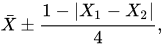
A fiducial or objective Bayesian argument can be used to derive the interval estimate $${\displaystyle {\bar {X}}\pm {\frac {1-|X_{1}-X_{2}|}{4}},}$$ which is also a 50% confidence procedure. Welch showed that the first confidence procedure dominates the second, according to desiderata from confidence interval theory; for every ${\displaystyle \theta _{1}\neq \theta }$, the probability that the first procedure contains ${\displaystyle \theta _{1}}$ is less than or equal to the probability that the second procedure contains ${\displaystyle \theta _{1}}$. The average width of the intervals from the first procedure is less than that of the second. Hence, the first procedure is preferred under classical confidence interval theory.

However, when ${\displaystyle |X_{1}-X_{2}|\geq 1/2}$, intervals from the first procedure are guaranteed to contain the true value ${\displaystyle \theta }$: Therefore, the nominal 50% confidence coefficient is unrelated to the uncertainty we should have that a specific interval contains the true value. The second procedure does not have this property.

Moreover, when the first procedure generates a very short interval, this indicates that ${\displaystyle X_{1},X_{2}}$ are very close together and hence only offer the information in a single data point. Yet the first interval will exclude almost all reasonable values of the parameter due to its short width. The second procedure does not have this property.

The two counter-intuitive properties of the first procedure – 100% coverage when ${\displaystyle X_{1},X_{2}}$ are far apart and almost 0% coverage when ${\displaystyle X_{1},X_{2}}$ are close together – balance out to yield 50% coverage on average. However, despite the first procedure being optimal, its intervals offer neither an assessment of the precision of the estimate nor an assessment of the uncertainty one should have that the interval contains the true value.

This example is used to argue against naïve interpretations of confidence intervals. If a confidence procedure is asserted to have properties beyond that of the nominal coverage (such as relation to precision, or a relationship with Bayesian inference), those properties must be proved; they do not follow from the fact that a procedure is a confidence procedure.

Steiger^[18] suggested a number of confidence procedures for common effect size measures in ANOVA. Morey et al.^[10] point out that several of these confidence procedures, including the one for ω², have the property that as the F statistic becomes increasingly small—indicating misfit with all possible values of ω²—the confidence interval shrinks and can even contain only the single value ω² = 0; that is, the CI is infinitesimally narrow (this occurs when ${\displaystyle p\geq 1-\alpha /2}$ for a ${\displaystyle 100(1-\alpha )\%}$ CI).

This behavior is consistent with the relationship between the confidence procedure and significance testing: as F becomes so small that the group means are much closer together than we would expect by chance, a significance test might indicate rejection for most or all values of ω². Hence the interval will be very narrow or even empty (or, by a convention suggested by Steiger, containing only 0). However, this does not indicate that the estimate of ω² is very precise. In a sense, it indicates the opposite: that the trustworthiness of the results themselves may be in doubt. This is contrary to the common interpretation of confidence intervals that they reveal the precision of the estimate.

Methods for calculating confidence intervals for the binomial proportion appeared from the 1920s.^[19][20] The main ideas of confidence intervals in general were developed in the early 1930s,^[21][22][23] and the first thorough and general account was given by Jerzy Neyman in 1937.^[7]

Neyman described the development of the ideas as follows (reference numbers have been changed):^[23]

[My work on confidence intervals] originated about 1930 from a simple question of Waclaw Pytkowski, then my student in Warsaw, engaged in an empirical study in farm economics. The question was: how to characterize non-dogmatically the precision of an estimated regression coefficient? ...

Pytkowski's monograph ... appeared in print in 1932.^[24] It so happened that, somewhat earlier, Fisher published his first paper^[25] concerned with fiducial distributions and fiducial argument. Quite unexpectedly, while the conceptual framework of fiducial argument is entirely different from that of confidence intervals, the specific solutions of several particular problems coincided. Thus, in the first paper in which I presented the theory of confidence intervals, published in 1934,^[21] I recognized Fisher's priority for the idea that interval estimation is possible without any reference to Bayes' theorem and with the solution being independent from probabilities a priori. At the same time I mildly suggested that Fisher's approach to the problem involved a minor misunderstanding.

In medical journals, confidence intervals were promoted in the 1970s but only became widely used in the 1980s.^[26] By 1988, medical journals were requiring the reporting of confidence intervals.^[27]

• Confidence interval for binomial distribution
• Confidence interval for exponent of the power law distribution
• Confidence interval for mean of the exponential distribution
• Confidence interval for mean of the Poisson distribution
• Confidence intervals for mean and variance of the normal distribution (also here)
• Confidence interval for the parameters of a simple linear regression
• Confidence interval for the difference of means (based on data from a normal distributions, without assuming equal variances)
• Confidence interval for the difference between two proportions

• CLs upper limits (particle physics)
• 68–95–99.7 rule
• Confidence band, an interval estimate for a curve
• Confidence distribution – Concept in statistics
• Confidence region – Multi-dimensional version of a confidence interval, a higher dimensional generalization
• Credence (statistics) – Measure of belief strength used in statistics
• Credible interval, a Bayesian alternative for interval estimation
• Cumulative distribution function-based nonparametric confidence interval – Class of confidence intervals around statistical functionals of a distribution
• Error bar – Graphical representations of the variability of data
• Estimation statistics – Data analysis approach in frequentist statistics
• Margin of error, the CI halfwidth
• p-value – Function of the observed sample results
• Prediction interval, an interval estimate for a random variable
• Probable error
• Robust confidence intervals – Statistical indicators of the deviation of a samplePages displaying short descriptions of redirect targets

Wikimedia Commons has media related to Confidence interval.

• The Exploratory Software for Confidence Intervals tutorial programs that run under Excel
• Confidence interval calculators for R-Squares, Regression Coefficients, and Regression Intercepts
• Weisstein, Eric W. "Confidence Interval". MathWorld.
• CAUSEweb.org Many resources for teaching statistics including Confidence Intervals.
• An interactive introduction to Confidence Intervals
• Confidence Intervals: Confidence Level, Sample Size, and Margin of Error by Eric Schulz, the Wolfram Demonstrations Project.
• Confidence Intervals in Public Health Archived 2016-08-09 at the Wayback Machine. Straightforward description with examples and what to do about small sample sizes or rates near 0.