Explore Black History

In statistics, a contingency table (also known as a cross tabulation or crosstab) is a type of table in a matrix format that displays the multivariate frequency distribution of the variables. They are heavily used in survey research, business intelligence, engineering, and scientific research. They provide a basic picture of the interrelation between two variables and can help find interactions between them. The term contingency table was first used by Karl Pearson in "On the Theory of Contingency and Its Relation to Association and Normal Correlation",^[1] part of the Drapers' Company Research Memoirs Biometric Series I published in 1904.

A crucial problem of multivariate statistics is finding the (direct-)dependence structure underlying the variables contained in high-dimensional contingency tables. If some of the conditional independences are revealed, then even the storage of the data can be done in a smarter way (see Lauritzen (2002)). In order to do this one can use information theory concepts, which gain the information only from the distribution of probability, which can be expressed easily from the contingency table by the relative frequencies.

A pivot table is a way to create contingency tables using spreadsheet software.

Suppose there are two variables, sex (male or female) and handedness (right- or left-handed). Further suppose that 100 individuals are randomly sampled from a very large population as part of a study of sex differences in handedness. A contingency table can be created to display the numbers of individuals who are male right-handed and left-handed, female right-handed and left-handed. Such a contingency table is shown below.

The numbers of the males, females, and right- and left-handed individuals are called marginal totals. The grand total (the total number of individuals represented in the contingency table) is the number in the bottom right corner.

The table allows users to see at a glance that the proportion of men who are right-handed is about the same as the proportion of women who are right-handed although the proportions are not identical. The strength of the association can be measured by the odds ratio, and the population odds ratio estimated by the sample odds ratio. The significance of the difference between the two proportions can be assessed with a variety of statistical tests including Pearson's chi-squared test, the G-test, Fisher's exact test, Boschloo's test, and Barnard's test, provided the entries in the table represent individuals randomly sampled from the population about which conclusions are to be drawn. If the proportions of individuals in the different columns vary significantly between rows (or vice versa), it is said that there is a contingency between the two variables. In other words, the two variables are not independent. If there is no contingency, it is said that the two variables are independent.

The example above is the simplest kind of contingency table, a table in which each variable has only two levels; this is called a 2 × 2 contingency table. In principle, any number of rows and columns may be used. There may also be more than two variables, but higher order contingency tables are difficult to represent visually. The relation between ordinal variables, or between ordinal and categorical variables, may also be represented in contingency tables, although such a practice is rare. For more on the use of a contingency table for the relation between two ordinal variables, see Goodman and Kruskal's gamma.

• Multiple columns (historically, they were designed to use up all the white space of a printed page). Where each row refers to a specific sub-group in the population (in this case men or women), the columns are sometimes referred to as banner points or cuts (and the rows are sometimes referred to as stubs).
• Significance tests. Typically, either column comparisons, which test for differences between columns and display these results using letters, or, cell comparisons, which use color or arrows to identify a cell in a table that stands out in some way.
• Nets or netts which are sub-totals.
• One or more of: percentages, row percentages, column percentages, indexes or averages.
• Unweighted sample sizes (counts).

The degree of association between the two variables can be assessed by a number of coefficients. The following subsections describe a few of them. For a more complete discussion of their uses, see the main articles linked under each subsection heading.

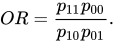
The simplest measure of association for a 2 × 2 contingency table is the odds ratio. Given two events, A and B, the odds ratio is defined as the ratio of the odds of A in the presence of B and the odds of A in the absence of B, or equivalently (due to symmetry), the ratio of the odds of B in the presence of A and the odds of B in the absence of A. Two events are independent if and only if the odds ratio is 1; if the odds ratio is greater than 1, the events are positively associated; if the odds ratio is less than 1, the events are negatively associated.

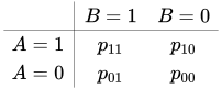
The odds ratio has a simple expression in terms of probabilities; given the joint probability distribution:

${\displaystyle {\begin{array}{c|cc}&B=1&B=0\\\hline A=1&p_{11}&p_{10}\\A=0&p_{01}&p_{00}\end{array}}}$

the odds ratio is:

${\displaystyle OR={\frac {p_{11}p_{00}}{p_{10}p_{01}}}.}$

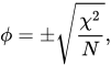
A simple measure, applicable only to the case of 2 × 2 contingency tables, is the phi coefficient (φ) defined by

${\displaystyle \phi =\pm {\sqrt {\frac {\chi ^{2}}{N}}},}$

where χ² is computed as in Pearson's chi-squared test, and N is the grand total of observations. φ varies from 0 (corresponding to no association between the variables) to 1 or −1 (complete association or complete inverse association), provided it is based on frequency data represented in 2 × 2 tables. Then its sign equals the sign of the product of the main diagonal elements of the table minus the product of the off–diagonal elements. φ takes on the minimum value −1.0 or the maximum value of +1.0 if and only if every marginal proportion is equal to 0.5 (and two diagonal cells are empty).^[2]

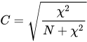
Two alternatives are the contingency coefficient C, and Cramér's V.

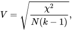
The formulae for the C and V coefficients are:

${\displaystyle C={\sqrt {\frac {\chi ^{2}}{N+\chi ^{2}}}}}$ and

${\displaystyle V={\sqrt {\frac {\chi ^{2}}{N(k-1)}}},}$

k being the number of rows or the number of columns, whichever is less.

C suffers from the disadvantage that it does not reach a maximum of 1.0, notably the highest it can reach in a 2 × 2 table is 0.707. It can reach values closer to 1.0 in contingency tables with more categories; for example, it can reach a maximum of 0.870 in a 4 × 4 table. It should, therefore, not be used to compare associations in different tables if they have different numbers of categories.^[3]

C can be adjusted so it reaches a maximum of 1.0 when there is complete association in a table of any number of rows and columns by dividing C by ${\displaystyle {\sqrt {\frac {k-1}{k}}}}$ where k is the number of rows or columns, when the table is square ^{[citation needed]}, or by ${\displaystyle {\sqrt[{\scriptstyle 4}]{{r-1 \over r}\times {c-1 \over c}}}}$ where r is the number of rows and c is the number of columns.^[4]

Another choice is the tetrachoric correlation coefficient but it is only applicable to 2 × 2 tables. Polychoric correlation is an extension of the tetrachoric correlation to tables involving variables with more than two levels.

Tetrachoric correlation assumes that the variable underlying each dichotomous measure is normally distributed.^[5] The coefficient provides "a convenient measure of [the Pearson product-moment] correlation when graduated measurements have been reduced to two categories."^[6]

The tetrachoric correlation coefficient should not be confused with the Pearson correlation coefficient computed by assigning, say, values 0.0 and 1.0 to represent the two levels of each variable (which is mathematically equivalent to the φ coefficient).

The lambda coefficient is a measure of the strength of association of the cross tabulations when the variables are measured at the nominal level. Values range from 0.0 (no association) to 1.0 (the maximum possible association).

Asymmetric lambda measures the percentage improvement in predicting the dependent variable. Symmetric lambda measures the percentage improvement when prediction is done in both directions.

The uncertainty coefficient, or Theil's U, is another measure for variables at the nominal level. Its values range from −1.0 (100% negative association, or perfect inversion) to +1.0 (100% positive association, or perfect agreement). A value of 0.0 indicates the absence of association.

Also, the uncertainty coefficient is conditional and an asymmetrical measure of association, which can be expressed as

${\displaystyle U(X|Y)\neq U(Y|X)}$.

This asymmetrical property can lead to insights not as evident in symmetrical measures of association.^[7]

Gamma, Tau-b and Tau-c are used when the categories or levels of both variables have a natural order.

• Gamma test: No adjustment for either table size or ties.
• Kendall's tau: Adjustment for ties.
  • Tau-b: Used for square tables.
  • Tau-c: Used for rectangular tables.

• Confusion matrix
• Pivot table, in spreadsheet software, cross-tabulates sampling data with counts (contingency table) and/or sums.
• TPL Tables is a tool for generating and printing crosstabs.
• The iterative proportional fitting procedure essentially manipulates contingency tables to match altered joint distributions or marginal sums.
• The multivariate statistics in special multivariate discrete probability distributions. Some procedures used in this context can be used in dealing with contingency tables.
• OLAP cube, a modern multidimensional computing form of contingency tables
• Panel data, multidimensional data over time

• Andersen, Erling B. 1980. Discrete Statistical Models with Social Science Applications. North Holland, 1980.
• Bishop, Y. M. M.; Fienberg, S. E.; Holland, P. W. (1975). Discrete Multivariate Analysis: Theory and Practice. MIT Press. ISBN 978-0-262-02113-5. MR 0381130.
• Christensen, Ronald (1997). Log-linear models and logistic regression. Springer Texts in Statistics (Second ed.). New York: Springer-Verlag. pp. xvi+483. ISBN 0-387-98247-7. MR 1633357.
• Lauritzen, Steffen L. (1979). Lectures on Contingency Tables (Aalborg University) (PDF) (4th edition (first electronic edition), 2002 ed.).
• Gokhale, D. V.; Kullback, Solomon (1978). The Information in Contingency Tables. Marcel Dekker. ISBN 0-824-76698-9.

Wikimedia Commons has media related to Contingency tables.

• On-line analysis of contingency tables: calculator with examples
• Interactive cross tabulation, chi-squared independent test, and tutorial
• Fisher and chi-squared calculator of 2 × 2 contingency table
• More Correlation Coefficients
• Nominal Association: Phi, Contingency Coefficient, Tschuprow's T, Cramer's V, Lambda, Uncertainty Coefficient, March 24, 2008, G. David Garson, North Carolina State University
• CustomInsight.com Cross Tabulation
• The POWERMUTT Project: IV. DISPLAYING CATEGORICAL DATA
• StATS: Steves Attempt to Teach Statistics Odds ratio versus relative risk (January 9, 2001)
• Epi Info Community Health Assessment Tutorial Lesson 5 Analysis: Creating Statistics