Civil Rights
Movements, leaders, victories and the continuing fight for equality.

Explore the people, places, events, achievements, struggles and stories that shaped our journey.
Movements, leaders, victories and the continuing fight for equality.
Innovation, patents, science, technology and world-changing contributions.
Pioneers, champions, Negro Leagues, records, activism and excellence.
Meet the people whose lives, choices and achievements shaped the journey.
Black towns, communities, institutions and places where history happened.
Moments that changed communities, movements, institutions and the nation.
Wilmington, North Carolina once had a thriving Black middle class and an elected interracial government. In 1898 white supremacists used violence to overthrow that government, kill Black residents and drive many others from the city.
MORE →Reflects the personal views, recollections, and perspective of the author, Mike Davis.
This is a personal recollection on the Move fire on May 13, 1985

In mathematics, deconvolution is the inverse of convolution. Both operations are used in signal processing and image processing. For example, it may be possible to recover the original signal after a filter (convolution) by using a deconvolution method with a certain degree of accuracy.[1] Due to the measurement error of the recorded signal or image, it can be demonstrated that the worse the signal-to-noise ratio (SNR), the worse the reversing of a filter will be; hence, inverting a filter is not always a good solution as the error amplifies. Deconvolution offers a solution to this problem.
The foundations for deconvolution and time-series analysis were largely laid by Norbert Wiener of the Massachusetts Institute of Technology in his book Extrapolation, Interpolation, and Smoothing of Stationary Time Series (1949).[2] The book was based on work Wiener had done during World War II but that had been classified at the time. Some of the early attempts to apply these theories were in the fields of weather forecasting and economics.
In general, the objective of deconvolution is to find the solution f of a convolution equation of the form:
Usually, h is some recorded signal, and f is some signal that we wish to recover, but has been convolved with a filter or distortion function g, before we recorded it. Usually, h is a distorted version of f and the shape of f can't be easily recognized by the eye or simpler time-domain operations. The function g represents the impulse response of an instrument or a driving force that was applied to a physical system. If we know g, or at least know the form of g, then we can perform deterministic deconvolution. However, if we do not know g in advance, then we need to estimate it. This can be done using methods of statistical estimation or building the physical principles of the underlying system, such as the electrical circuit equations or diffusion equations.
There are several deconvolution techniques, depending on the choice of the measurement error and deconvolution parameters:
When the measurement error is very low (ideal case), deconvolution collapses into a filter reversing. This kind of deconvolution can be performed in the Laplace domain. By computing the Fourier transform of the recorded signal h and the system response function g, you get H and G, with G as the transfer function. Using the convolution theorem,
where F is the estimated Fourier transform of f. Finally, the inverse Fourier transform of the function F is taken to find the estimated deconvolved signal f. Note that G is at the denominator and could amplify elements of the error model if present.
In physical measurements, the situation is usually closer to
In this case ε is noise that has entered our recorded signal. If a noisy signal or image is assumed to be noiseless, the statistical estimate of g will be incorrect. In turn, the estimate of ƒ will also be incorrect. The lower the signal-to-noise ratio, the worse the estimate of the deconvolved signal will be. That is the reason why inverse filtering the signal (as in the "raw deconvolution" above) is usually not a good solution. However, if at least some knowledge exists of the type of noise in the data (for example, white noise), the estimate of ƒ can be improved through techniques such as Wiener deconvolution.
A direct time-domain method can be formulated for non-cyclic (linear) convolution.[3][4] Let
where and are known and is to be determined. Define
Then
With the change of variable ,
For odd , therefore,
and hence
Thus the operation generates zeros between the nonzero elements of the convolution kernel.[3]
Repeating the sign-change and convolution operations increases the spacing between the remaining nonzero elements of the convolution kernel. After such stages, each remaining nonzero element is followed by zeros. For finite non-cyclic convolution, these separated nonzero coefficients can be regarded as scaled delta functions, which produce corresponding groups in the transformed output. Each group gives the impulse response after division by the coefficient of the delta function that produces it.[3]
For example, let
and
Their non-cyclic convolution is
After two stages, the equivalent convolution kernel is
and the corresponding transformed output is
Since , three zeros separate successive nonzero coefficients of the convolution kernel. The four coefficients produce four corresponding output groups. The first two are[3]
and
Dividing each group by the coefficient of the delta function that produces it recovers
The concept of deconvolution had an early application in reflection seismology. In 1950, Enders Robinson was a graduate student at MIT. He worked with others at MIT, such as Norbert Wiener, Norman Levinson, and economist Paul Samuelson, to develop the "convolutional model" of a reflection seismogram. This model assumes that the recorded seismogram s(t) is the convolution of an Earth-reflectivity function e(t) and a seismic wavelet w(t) from a point source, where t represents recording time. Thus, our convolution equation is
The seismologist is interested in e, which contains information about the Earth's structure. By the convolution theorem, this equation may be Fourier transformed to
in the frequency domain, where is the frequency variable. By assuming that the reflectivity is white, we can assume that the power spectrum of the reflectivity is constant, and that the power spectrum of the seismogram is the spectrum of the wavelet multiplied by that constant. Thus,
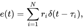
If we assume that the wavelet is minimum phase, we can recover it by calculating the minimum phase equivalent of the power spectrum we just found. The reflectivity may be recovered by designing and applying a Wiener filter that shapes the estimated wavelet to a Dirac delta function (i.e., a spike). The result may be seen as a series of scaled, shifted delta functions (although this is not mathematically rigorous):
where N is the number of reflection events, are the reflection coefficients, are the reflection times of each event, and is the Dirac delta function.
In practice, since we are dealing with noisy, finite bandwidth, finite length, discretely sampled datasets, the above procedure only yields an approximation of the filter required to deconvolve the data. However, by formulating the problem as the solution of a Toeplitz matrix and using Levinson recursion, we can relatively quickly estimate a filter with the smallest mean squared error possible. We can also do deconvolution directly in the frequency domain and get similar results. The technique is closely related to linear prediction.

In optics and imaging, the term "deconvolution" is specifically used to refer to the process of reversing the optical distortion that takes place in an optical microscope, electron microscope, telescope, or other imaging instrument, thus creating clearer images. It is usually done in the digital domain by a software algorithm, as part of a suite of microscope image processing techniques. Deconvolution is also practical to sharpen images that suffer from fast motion or jiggles during capturing. Early Hubble Space Telescope images were distorted by a flawed mirror and were sharpened by deconvolution.
The usual method is to assume that the optical path through the instrument is optically perfect, convolved with a point spread function (PSF), that is, a mathematical function that describes the distortion in terms of the pathway a theoretical point source of light (or other waves) takes through the instrument.[5] Usually, such a point source contributes a small area of fuzziness to the final image. If this function can be determined, it is then a matter of computing its inverse or complementary function, and convolving the acquired image with that. The result is the original, undistorted image.
In practice, finding the true PSF is impossible, and usually an approximation of it is used, theoretically calculated[6] or based on some experimental estimation by using known probes. Real optics may also have different PSFs at different focal and spatial locations, and the PSF may be non-linear. The accuracy of the approximation of the PSF will dictate the final result. Different algorithms can be employed to give better results, at the price of being more computationally intensive. Since the original convolution discards data, some algorithms use additional data acquired at nearby focal points to make up some of the lost information. Regularization in iterative algorithms (as in expectation-maximization algorithms) can be applied to avoid unrealistic solutions.
When the PSF is unknown, it may be possible to deduce it by systematically trying different possible PSFs and assessing whether the image has improved. This procedure is called blind deconvolution.[5] Blind deconvolution is a well-established image restoration technique in astronomy, where the point nature of the objects photographed exposes the PSF thus making it more feasible. It is also used in fluorescence microscopy for image restoration, and in fluorescence spectral imaging for spectral separation of multiple unknown fluorophores. The most common iterative algorithm for the purpose is the Richardson–Lucy deconvolution algorithm; the Wiener deconvolution (and approximations) are the most common non-iterative algorithms.

For some specific imaging systems such as laser pulsed terahertz systems, PSF can be modeled mathematically.[8] As a result, as shown in the figure, deconvolution of the modeled PSF and the terahertz image can give a higher resolution representation of the terahertz image.
When performing image synthesis in radio interferometry, a specific kind of radio astronomy, one step consists of deconvolving the produced image with the "dirty beam", which is a different name for the point spread function. A commonly used method is the CLEAN algorithm.
Typical use of deconvolution is in tracer kinetics. For example, when measuring a hormone concentration in the blood, its secretion rate can be estimated by deconvolution. Another example is the estimation of the blood glucose concentration from the measured interstitial glucose, which is a distorted version in time and amplitude of the real blood glucose.[9]
Deconvolution has been applied extensively to absorption spectra.[10] The Van Cittert algorithm (article in German) may be used.[11]
Deconvolution maps to division in the Fourier co-domain. This allows deconvolution to be easily applied with experimental data that are subject to a Fourier transform. An example is NMR spectroscopy where the data are recorded in the time domain, but analyzed in the frequency domain. Division of the time-domain data by an exponential function has the effect of reducing the width of Lorentzian lines in the frequency domain.
{{cite book}}: ISBN / Date incompatibility (help)
| International | |
|---|---|
| National | |
| Other | |
Source: Wikipedia. Article content is retrieved live through the MediaWiki API.

In mathematics, deconvolution is the inverse of convolution. Both operations are used in signal processing and image processing. For example, it may be possible to recover the original signal after a filter (convolution) by using a deconvolution method with a certain degree of accuracy. Due to the measurement error of the recorded signal or image, it can be demonstrated that the worse the signal-to-noise ratio (SNR), the worse the reversing of a filter will be; hence, inverting a filter is not always a good solution as the error amplifies. Deconvolution offers a solution to this problem. The foundations for deconvolution and time-series analysis were largely laid by Norbert Wiener of the Massachusetts Institute of Technology in his book Extrapolation, Interpolation, and Smoothing of Stationary Time Series (1949). The book was based on work Wiener had done during World War II but that had been classified at the time. Some of the early attempts to apply these theories were in the fields of weather forecasting and economics.

The Richardson–Lucy algorithm, also known as Lucy–Richardson deconvolution, is an iterative procedure for recovering an underlying image that has been blurred by a known point spread function. It was named after William Richardson and Leon B. Lucy, who described it independently.

In electrical engineering and applied mathematics, blind deconvolution is deconvolution without explicit knowledge of the impulse response function used in the convolution. This is usually achieved by making appropriate assumptions of the input to estimate the impulse response by analyzing the output. Blind deconvolution is not solvable without making assumptions on input and impulse response. Most of the algorithms to solve this problem are based on assumption that both input and impulse response live in respective known subspaces. However, blind deconvolution remains a very challenging non-convex optimization problem even with this assumption.

In mathematics, Wiener deconvolution is an application of the Wiener filter to the noise problems inherent in deconvolution. It works in the frequency domain, attempting to minimize the impact of deconvolved noise at frequencies which have a poor signal-to-noise ratio. The Wiener deconvolution method has widespread use in image deconvolution applications, as the frequency spectrum of most visual images is fairly well behaved and may be estimated easily. Wiener deconvolution is named after Norbert Wiener.
Before the 1921 destruction of Tulsa’s Greenwood District, Black residents had created a remarkable center of business and community life. The district included stores, professional offices, entertainment venues and homes owned by Black citizens. Understanding Greenwood means learning what was built—not only what was burned.
MORE →Brown v. Board of Education in 1954.