Explore Black History

This article includes a list of general references but lacks sufficient corresponding inline citations. Please help improve this article by introducing more precise citations. (June 2025) (Learn how and when to remove this message)

In linear algebra, a diagonal matrix is a matrix in which the entries outside the main diagonal are all zero; the term usually refers to square matrices. Elements of the main diagonal can either be zero or nonzero. An example of a 2×2 diagonal matrix is ${\displaystyle \left[{\begin{smallmatrix}3&0\\0&2\end{smallmatrix}}\right]}$, while an example of a 3×3 diagonal matrix is${\displaystyle \left[{\begin{smallmatrix}6&0&0\\0&5&0\\0&0&4\end{smallmatrix}}\right]}$. An identity matrix of any size, or any multiple of it is a diagonal matrix called a scalar matrix, for example, ${\displaystyle \left[{\begin{smallmatrix}0.5&0\\0&0.5\end{smallmatrix}}\right]}$. In geometry, a diagonal matrix may be used as a scaling matrix, since matrix multiplication with it results in changing scale (size) and possibly also shape; only a scalar matrix results in uniform change in scale.

As stated above, a diagonal matrix is a matrix in which all off-diagonal entries are zero. That is, the matrix D = (d_i,j) with n columns and n rows is diagonal if $${\displaystyle \forall i,j\in \{1,2,\ldots ,n\},i\neq j\implies d_{i,j}=0.}$$

However, the main diagonal entries are unrestricted.

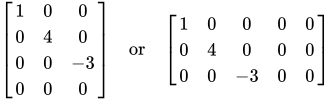
The term diagonal matrix may sometimes refer to a rectangular diagonal matrix, which is an m-by-n matrix with all the entries not of the form d_i,i being zero. For example: $${\displaystyle {\begin{bmatrix}1&0&0\\0&4&0\\0&0&-3\\0&0&0\\\end{bmatrix}}\quad {\text{or}}\quad {\begin{bmatrix}1&0&0&0&0\\0&4&0&0&0\\0&0&-3&0&0\end{bmatrix}}}$$

More often, however, diagonal matrix refers to square matrices, which can be specified explicitly as a square diagonal matrix. A square diagonal matrix is a symmetric matrix, so this can also be called a symmetric diagonal matrix.

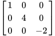
The following matrix is square diagonal matrix: $${\displaystyle {\begin{bmatrix}1&0&0\\0&4&0\\0&0&-2\end{bmatrix}}}$$

If the entries are real numbers or complex numbers, then it is a normal matrix as well.

In the remainder of this article we will consider only square diagonal matrices, and refer to them simply as "diagonal matrices".

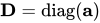
A diagonal matrix D can be constructed from a vector ${\displaystyle \mathbf {a} ={\begin{bmatrix}a_{1}&\dots &a_{n}\end{bmatrix}}^{\textsf {T}}}$ using the ${\displaystyle \operatorname {diag} }$ operator: $${\displaystyle \mathbf {D} =\operatorname {diag} (a_{1},\dots ,a_{n}).}$$

This may be written more compactly as ${\displaystyle \mathbf {D} =\operatorname {diag} (\mathbf {a} )}$.

The same operator is also used to represent block diagonal matrices as ${\displaystyle \mathbf {A} =\operatorname {diag} (\mathbf {A} _{1},\dots ,\mathbf {A} _{n})}$ where each argument A_i is a matrix.

The diag operator may be written as $${\displaystyle \operatorname {diag} (\mathbf {a} )=\left(\mathbf {a} \mathbf {1} ^{\textsf {T}}\right)\circ \mathbf {I} ,}$$ where ${\displaystyle \circ }$ represents the Hadamard product, and 1 is a constant vector with elements 1.

The inverse matrix-to-vector diag operator is sometimes denoted by the identically named ${\displaystyle \operatorname {diag} (\mathbf {D} )={\begin{bmatrix}a_{1}&\dots &a_{n}\end{bmatrix}}^{\textsf {T}},}$ where the argument is now a matrix, and the result is a vector of its diagonal entries.

The following property holds: $${\displaystyle \operatorname {diag} (\mathbf {A} \mathbf {B} )=\sum _{j}\left(\mathbf {A} \circ \mathbf {B} ^{\textsf {T}}\right)_{ij}=\left(\mathbf {A} \circ \mathbf {B} ^{\textsf {T}}\right)\mathbf {1} .}$$

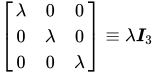
A diagonal matrix with equal diagonal entries is a scalar matrix; that is, a scalar multiple λ of the identity matrix I. Its effect on a vector is scalar multiplication by λ. For example, a 3×3 scalar matrix has the form: $${\displaystyle {\begin{bmatrix}\lambda &0&0\\0&\lambda &0\\0&0&\lambda \end{bmatrix}}\equiv \lambda {\boldsymbol {I}}_{3}}$$

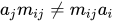
The scalar matrices are the center of the algebra of matrices: that is, they are precisely the matrices that commute with all other square matrices of the same size.^[a] By contrast, over a field (like the real numbers), a diagonal matrix with all diagonal elements distinct only commutes with diagonal matrices (its centralizer is the set of diagonal matrices). That is because if a diagonal matrix ${\displaystyle \mathbf {D} =\operatorname {diag} (a_{1},\dots ,a_{n})}$ has ${\displaystyle a_{i}\neq a_{j},}$ then given a matrix M with ${\displaystyle m_{ij}\neq 0,}$ the (i, j) term of the products are: ${\displaystyle (\mathbf {DM} )_{ij}=a_{i}m_{ij}}$ and ${\displaystyle (\mathbf {MD} )_{ij}=m_{ij}a_{j},}$ and ${\displaystyle a_{j}m_{ij}\neq m_{ij}a_{i}}$ (since one can divide by m_ij), so they do not commute unless the off-diagonal terms are zero.^[b] Diagonal matrices where the diagonal entries are not all equal or all distinct have centralizers intermediate between the whole space and only diagonal matrices.^[1]

For an abstract vector space V (rather than the concrete vector space Kⁿ), the analog of scalar matrices are scalar transformations. This is true more generally for a module M over a ring R, with the endomorphism algebra End(M) (algebra of linear operators on M) replacing the algebra of matrices. Formally, scalar multiplication is a linear map, inducing a map ${\displaystyle R\to \operatorname {End} (M),}$ (from a scalar λ to its corresponding scalar transformation, multiplication by λ) exhibiting End(M) as a R-algebra. For vector spaces, the scalar transforms are exactly the center of the endomorphism algebra, and, similarly, scalar invertible transforms are the center of the general linear group GL(V). The former is more generally true free modules ${\displaystyle M\cong R^{n},}$ for which the endomorphism algebra is isomorphic to a matrix algebra.

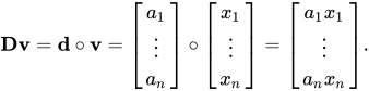
Multiplying a vector by a diagonal matrix multiplies each of the terms by the corresponding diagonal entry. Given a diagonal matrix ${\displaystyle \mathbf {D} =\operatorname {diag} (a_{1},\dots ,a_{n})}$ and a vector ${\displaystyle \mathbf {v} ={\begin{bmatrix}x_{1}&\dotsm &x_{n}\end{bmatrix}}^{\textsf {T}}}$, the product is: $${\displaystyle \mathbf {D} \mathbf {v} =\operatorname {diag} (a_{1},\dots ,a_{n}){\begin{bmatrix}x_{1}\\\vdots \\x_{n}\end{bmatrix}}={\begin{bmatrix}a_{1}\\&\ddots \\&&a_{n}\end{bmatrix}}{\begin{bmatrix}x_{1}\\\vdots \\x_{n}\end{bmatrix}}={\begin{bmatrix}a_{1}x_{1}\\\vdots \\a_{n}x_{n}\end{bmatrix}}.}$$

This can be expressed more compactly by using a vector instead of a diagonal matrix, ${\displaystyle \mathbf {d} ={\begin{bmatrix}a_{1}&\dotsm &a_{n}\end{bmatrix}}^{\textsf {T}}}$, and taking the Hadamard product of the vectors (entrywise product), denoted ${\displaystyle \mathbf {d} \circ \mathbf {v} }$:

$${\displaystyle \mathbf {D} \mathbf {v} =\mathbf {d} \circ \mathbf {v} ={\begin{bmatrix}a_{1}\\\vdots \\a_{n}\end{bmatrix}}\circ {\begin{bmatrix}x_{1}\\\vdots \\x_{n}\end{bmatrix}}={\begin{bmatrix}a_{1}x_{1}\\\vdots \\a_{n}x_{n}\end{bmatrix}}.}$$

This is mathematically equivalent, but avoids storing all the zero terms of this sparse matrix. This product is thus used in machine learning, such as computing products of derivatives in backpropagation or multiplying IDF weights in TF-IDF,^[2] since some BLAS frameworks, which multiply matrices efficiently, do not include Hadamard product capability directly.^[3]

The operations of matrix addition and matrix multiplication are especially simple for diagonal matrices. Write diag(a₁, ..., a_n) for a diagonal matrix whose diagonal entries starting in the upper left corner are a₁, ..., a_n. Then, for addition, we have

$${\displaystyle \operatorname {diag} (a_{1},\,\ldots ,\,a_{n})+\operatorname {diag} (b_{1},\,\ldots ,\,b_{n})=\operatorname {diag} (a_{1}+b_{1},\,\ldots ,\,a_{n}+b_{n})}$$

and for matrix multiplication,

$${\displaystyle \operatorname {diag} (a_{1},\,\ldots ,\,a_{n})\operatorname {diag} (b_{1},\,\ldots ,\,b_{n})=\operatorname {diag} (a_{1}b_{1},\,\ldots ,\,a_{n}b_{n}).}$$

The diagonal matrix diag(a₁, ..., a_n) is invertible if and only if the entries a₁, ..., a_n are all nonzero. In this case, we have

$${\displaystyle \operatorname {diag} (a_{1},\,\ldots ,\,a_{n})^{-1}=\operatorname {diag} (a_{1}^{-1},\,\ldots ,\,a_{n}^{-1}).}$$

In particular, the diagonal matrices form a subring of the ring of all n-by-n matrices.

Multiplying an n-by-n matrix A from the left with diag(a₁, ..., a_n) amounts to multiplying the i-th row of A by a_i for all i; multiplying the matrix A from the right with diag(a₁, ..., a_n) amounts to multiplying the i-th column of A by a_i for all i.

As explained in determining coefficients of operator matrix, there is a special basis, e₁, ..., e_n, for which the matrix A takes the diagonal form. Hence, in the defining equation ${\textstyle \mathbf {Ae} _{j}=\sum _{i}a_{i,j}\mathbf {e} _{i}}$, all coefficients a_{i, j} with i ≠ j are zero, leaving only one term per sum. The surviving diagonal elements, a_{i, j}, are known as eigenvalues and designated with λ_i in the equation, which reduces to ${\displaystyle \mathbf {Ae} _{i}=\lambda _{i}\mathbf {e} _{i}.}$ The resulting equation is known as eigenvalue equation^[4] and used to derive the characteristic polynomial and, further, eigenvalues and eigenvectors.

In other words, the eigenvalues of diag(λ₁, ..., λ_n) are λ₁, ..., λ_n with associated eigenvectors of e₁, ..., e_n.

• The determinant of diag(a₁, ..., a_n) is the product a₁⋯a_n.
• The adjugate of a diagonal matrix is again diagonal.
• Where all matrices are square,
  • A matrix is diagonal if and only if it is triangular and normal.
  • A matrix is diagonal if and only if it is both upper- and lower-triangular.
  • A diagonal matrix is symmetric.
• The identity matrix I_n and zero matrix are diagonal.
• A 1×1 matrix is always diagonal.
• The square of a 2×2 matrix with zero trace is always diagonal.
• The inverse of a diagonal matrix is obtained by taking the reciprocals of the elements on the diagonal

Diagonal matrices occur in many areas of linear algebra. Because of the simple description of the matrix operation and eigenvalues/eigenvectors given above, it is typically desirable to represent a given matrix or linear map by a diagonal matrix.

In fact, a given n-by-n matrix A is similar to a diagonal matrix (meaning that there is a matrix X such that X⁻¹AX is diagonal) if and only if it has n linearly independent eigenvectors. Such matrices are said to be diagonalizable.

Over the field of real or complex numbers, more is true. The spectral theorem says that every normal matrix is unitarily similar to a diagonal matrix (if AA^∗ = A^∗A then there exists a unitary matrix U such that UAU^∗ is diagonal). Furthermore, the singular value decomposition implies that for any matrix A, there exist unitary matrices U and V such that U^∗AV is diagonal with positive entries.

In operator theory, particularly the study of PDEs, operators are particularly easy to understand and PDEs easy to solve if the operator is diagonal with respect to the basis with which one is working; this corresponds to a separable partial differential equation. Therefore, a key technique to understanding operators is a change of coordinates—in the language of operators, an integral transform—which changes the basis to an eigenbasis of eigenfunctions: which makes the equation separable. An important example of this is the Fourier transform, which diagonalizes constant coefficient differentiation operators (or more generally translation invariant operators), such as the Laplacian operator, say, in the heat equation.

Especially easy are multiplication operators, which are defined as multiplication by (the values of) a fixed function–the values of the function at each point correspond to the diagonal entries of a matrix.

• Horn, Roger Alan; Johnson, Charles Royal (1985), Matrix Analysis, Cambridge University Press, ISBN 978-0-521-38632-6