Explore Black History

In statistics, Hodges' estimator^[1] (or the Hodges–Le Cam estimator^[2]), named for Joseph Hodges, is a famous counterexample demonstrating the existence of an estimator which is "superefficient",^[3] i.e. it attains smaller asymptotic variance than regular efficient estimators. The existence of such a counterexample is the reason for the introduction of the notion of regular estimators.

Hodges' estimator improves upon a regular estimator at a single point. In general, any superefficient estimator may surpass a regular estimator at most on a set of Lebesgue measure zero.^[4]

Although Hodges discovered the estimator he never published it; the first publication was in the doctoral thesis of Lucien Le Cam.^[5]

Suppose ${\displaystyle {\hat {\theta }}_{n}}$ is a "common" estimator for some parameter ${\displaystyle \theta }$: it is consistent, and converges to some asymptotic distribution ${\displaystyle L_{\theta }}$ (usually this is a normal distribution with mean zero and variance which may depend on ${\displaystyle \theta }$) at the ${\displaystyle {\sqrt {n}}}$-rate:

${\displaystyle {\sqrt {n}}({\hat {\theta }}_{n}-\theta )\ {\xrightarrow {d}}\ L_{\theta }\ .}$

Then the Hodges' estimator ${\displaystyle {\hat {\theta }}_{n}^{H}}$ is defined as^[6]

${\displaystyle {\hat {\theta }}_{n}^{H}={\begin{cases}{\hat {\theta }}_{n},&{\text{if }}|{\hat {\theta }}_{n}|\geq n^{-1/4},{\text{ and}}\\0,&{\text{if }}|{\hat {\theta }}_{n}|<n^{-1/4}.\end{cases}}}$

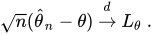
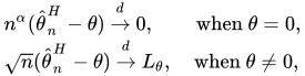
This estimator is equal to ${\displaystyle {\hat {\theta }}_{n}}$ everywhere except on the small interval ${\displaystyle [-n^{-1/4},n^{-1/4}]}$, where it is equal to zero. It is not difficult to see that this estimator is consistent for ${\displaystyle \theta }$, and its asymptotic distribution is^[7]

${\displaystyle {\begin{aligned}&n^{\alpha }({\hat {\theta }}_{n}^{H}-\theta )\ {\xrightarrow {d}}\ 0,\qquad {\text{when }}\theta =0,\\&{\sqrt {n}}({\hat {\theta }}_{n}^{H}-\theta )\ {\xrightarrow {d}}\ L_{\theta },\quad {\text{when }}\theta \neq 0,\end{aligned}}}$

for any ${\displaystyle \alpha \in \mathbb {R} }$. Thus this estimator has the same asymptotic distribution as ${\displaystyle {\hat {\theta }}_{n}}$ for all ${\displaystyle \theta \neq 0}$, whereas for ${\displaystyle \theta =0}$ the rate of convergence becomes arbitrarily fast. This estimator is superefficient, as it surpasses the asymptotic behavior of the efficient estimator ${\displaystyle {\hat {\theta }}_{n}}$ at least at one point ${\displaystyle \theta =0}$.

It is not true that the Hodges estimator is equivalent to the sample mean, but much better when the true mean is 0. The correct interpretation is that, for finite ${\displaystyle n}$, the truncation can lead to worse square error than the sample mean estimator for ${\displaystyle E[X]}$ close to 0, as is shown in the example in the following section.^[8]

Le Cam shows that this behaviour is typical: superefficiency at the point θ implies the existence of a sequence ${\displaystyle \theta _{n}\rightarrow \theta }$ such that ${\displaystyle \liminf _{n\to \infty }E\theta _{n}\ell ({\sqrt {n}}({\hat {\theta }}_{n}-\theta _{n}))}$ is strictly larger than the Cramér–Rao bound. For the extreme case where the asymptotic risk at θ is zero, the ${\displaystyle \liminf _{n\to \infty }}$ is even infinite for a sequence ${\displaystyle \theta _{n}\rightarrow \theta }$.^[9]

In general, superefficiency may only be attained on a subset of Lebesgue measure zero of the parameter space ${\displaystyle \Theta }$.^[10]

Suppose x₁, ..., x_n is an independent and identically distributed (IID) random sample from normal distribution N(θ, 1) with unknown mean but known variance. Then the common estimator for the population mean θ is the arithmetic mean of all observations: ${\displaystyle {\bar {x}}}$. The corresponding Hodges' estimator will be ${\displaystyle {\hat {\theta }}_{n}^{H}\;=\;{\bar {x}}\cdot \mathbf {1} \{|{\bar {x}}|\,\geq \,n^{-1/4}\}}$, where 1{...} denotes the indicator function.

The mean square error (scaled by n) associated with the regular estimator x is constant and equal to 1 for all θ's. At the same time the mean square error of the Hodges' estimator ${\displaystyle {\hat {\theta }}_{n}^{H}}$ behaves erratically in the vicinity of zero, and even becomes unbounded as n → ∞. This demonstrates that the Hodges' estimator is not regular, and its asymptotic properties are not adequately described by limits of the form (θ fixed, n → ∞).

• James–Stein estimator