Explore Black History

The Ford–Fulkerson method or Ford–Fulkerson algorithm (FFA) is a greedy algorithm that computes the maximum flow in a flow network. It is sometimes called a "method" instead of an "algorithm" as the approach to finding augmenting paths in a residual graph is not fully specified^[1] or it is specified in several implementations with different running times.^[2] It was published in 1956 by L. R. Ford Jr. and D. R. Fulkerson.^[3] The name "Ford–Fulkerson" is often also used for the Edmonds–Karp algorithm, which is a fully defined implementation of the Ford–Fulkerson method.

The idea behind the algorithm is as follows: as long as there is a path from the source (start node) to the sink (end node), with available capacity on all edges in the path, we send flow along one of the paths. Then we find another path, and so on. A path with available capacity is called an augmenting path.

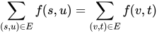
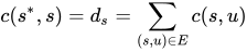
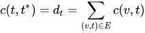
Let ${\displaystyle G(V,E)}$ be a graph, and for each edge from u to v, let ${\displaystyle c(u,v)}$ be the capacity and ${\displaystyle f(u,v)}$ be the flow. We want to find the maximum flow from the source s to the sink t. After every step in the algorithm the following is maintained:

Capacity constraints	${\displaystyle \forall (u,v)\in E:\ f(u,v)\leq c(u,v)}$	The flow along an edge cannot exceed its capacity.
Skew symmetry	${\displaystyle \forall (u,v)\in E:\ f(u,v)=-f(v,u)}$	The net flow from u to v must be the opposite of the net flow from v to u (see example).
Flow conservation	${\displaystyle \forall u\in V:u\neq s{\text{ and }}u\neq t\Rightarrow \sum _{w\in V}f(u,w)=0}$	The net flow to a node is zero, except for the source, which "produces" flow, and the sink, which "consumes" flow.
Value(f)	${\displaystyle \sum _{(s,u)\in E}f(s,u)=\sum _{(v,t)\in E}f(v,t)}$	The flow leaving from s must be equal to the flow arriving at t.

This means that the flow through the network is a legal flow after each round in the algorithm. We define the residual network ${\displaystyle G_{f}(V,E_{f})}$ to be the network with capacity ${\displaystyle c_{f}(u,v)=c(u,v)-f(u,v)}$ and no flow. Notice that it can happen that a flow from v to u is allowed in the residual network, though disallowed in the original network: if ${\displaystyle f(u,v)>0}$ and ${\displaystyle c(v,u)=0}$ then ${\displaystyle c_{f}(v,u)=c(v,u)-f(v,u)=f(u,v)>0}$.

Algorithm Ford–Fulkerson

The path in step 2 can be found with, for example, breadth-first search (BFS) or depth-first search in ${\displaystyle G_{f}(V,E_{f})}$. The former is known as the Edmonds–Karp algorithm.

When no more paths in step 2 can be found, s will not be able to reach t in the residual network. If S is the set of nodes reachable by s in the residual network, then the total capacity in the original network of edges from S to the remainder of V is on the one hand equal to the total flow we found from s to t, and on the other hand serves as an upper bound for all such flows. This proves that the flow we found is maximal. See also Max-flow Min-cut theorem.

If the graph ${\displaystyle G(V,E)}$ has multiple sources and sinks, we act as follows: Suppose that ${\displaystyle T=\{t\mid t{\text{ is a sink}}\}}$ and ${\displaystyle S=\{s\mid s{\text{ is a source}}\}}$. Add a new source ${\displaystyle s^{*}}$ with an edge ${\displaystyle (s^{*},s)}$ from ${\displaystyle s^{*}}$ to every node ${\displaystyle s\in S}$, with capacity ${\displaystyle c(s^{*},s)=d_{s}=\sum _{(s,u)\in E}c(s,u)}$. And add a new sink ${\displaystyle t^{*}}$ with an edge ${\displaystyle (t,t^{*})}$ from every node ${\displaystyle t\in T}$ to ${\displaystyle t^{*}}$, with capacity ${\displaystyle c(t,t^{*})=d_{t}=\sum _{(v,t)\in E}c(v,t)}$. Then apply the Ford–Fulkerson algorithm.

Also, if a node u has capacity constraint ${\displaystyle d_{u}}$, we replace this node with two nodes ${\displaystyle u_{\mathrm {in} },u_{\mathrm {out} }}$, and an edge ${\displaystyle (u_{\mathrm {in} },u_{\mathrm {out} })}$, with capacity ${\displaystyle c(u_{\mathrm {in} },u_{\mathrm {out} })=d_{u}}$. We can then apply the Ford–Fulkerson algorithm.

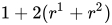
By adding the flow augmenting path to the flow already established in the graph, the maximum flow will be reached when no more flow augmenting paths can be found in the graph. However, there is no certainty that this situation will ever be reached, so the best that can be guaranteed is that the answer will be correct if the algorithm terminates. In the case that the algorithm does not terminate, the flow might not converge towards the maximum flow. However, this situation only occurs with irrational flow values.^[4] When the capacities are integers, the runtime of Ford–Fulkerson is bounded by ${\displaystyle O(Ef)}$ (see big O notation), where ${\displaystyle E}$ is the number of edges in the graph and ${\displaystyle f}$ is the maximum flow in the graph. This is because each augmenting path can be found in ${\displaystyle O(E)}$ time and increases the flow by an integer amount of at least ${\displaystyle 1}$, with the upper bound ${\displaystyle f}$.

A variation of the Ford–Fulkerson algorithm with guaranteed termination and a runtime independent of the maximum flow value is the Edmonds–Karp algorithm, which runs in ${\displaystyle O(VE^{2})}$ time.

The following example shows the first steps of Ford–Fulkerson in a flow network with 4 nodes, source ${\displaystyle A}$ and sink ${\displaystyle D}$. This example shows the worst-case behaviour of the algorithm. In each step, only a flow of ${\displaystyle 1}$ is sent across the network. If breadth-first-search were used instead, only two steps would be needed.

Step	Flow network
Initial flow network.
Flow is sent along the augmenting path ${\displaystyle A,B,C,D}$. Here, the bottleneck is the ${\displaystyle B}$–${\displaystyle C}$ edge, so only one unit of flow is possible.
Here, one unit of flow is sent along the augmenting path ${\displaystyle A,C,B,D}$. In this case, flow is "pushed back" from ${\displaystyle C}$ to ${\displaystyle B}$. The flow into ${\displaystyle C}$ that originally came from ${\displaystyle B}$ now comes from ${\displaystyle A}$, and ${\displaystyle B}$ is now free to send flow to ${\displaystyle D}$ directly. As a result, the ${\displaystyle B}$–${\displaystyle C}$ edge is left with zero flow, but the overall flow increases by one.
1998 intermediate steps are omitted here.
The final flow network, with a total flow of 2000 units.

Consider the flow network shown on the right, with source ${\displaystyle s}$, sink ${\displaystyle t}$, capacities of edges ${\displaystyle e_{1}=1}$, ${\displaystyle e_{2}=r=({\sqrt {5}}-1)/2}$ and ${\displaystyle e_{3}=1}$, and the capacity of all other edges some integer ${\displaystyle M\geq 2}$. The constant ${\displaystyle r}$ was chosen so, that ${\displaystyle r^{2}=1-r}$. We use augmenting paths according to the following table, where ${\displaystyle p_{1}=\{s,v_{4},v_{3},v_{2},v_{1},t\}}$, ${\displaystyle p_{2}=\{s,v_{2},v_{3},v_{4},t\}}$ and ${\displaystyle p_{3}=\{s,v_{1},v_{2},v_{3},t\}}$.

Step	Augmenting path	Sent flow	Residual capacities
			${\displaystyle e_{1}}$	${\displaystyle e_{2}}$	${\displaystyle e_{3}}$
0			${\displaystyle r^{0}=1}$	${\displaystyle r}$	${\displaystyle 1}$
1	${\displaystyle \{s,v_{2},v_{3},t\}}$	${\displaystyle 1}$	${\displaystyle r^{0}}$	${\displaystyle r^{1}}$	${\displaystyle 0}$
2	${\displaystyle p_{1}}$	${\displaystyle r^{1}}$	${\displaystyle r^{0}-r^{1}=r^{2}}$	${\displaystyle 0}$	${\displaystyle r^{1}}$
3	${\displaystyle p_{2}}$	${\displaystyle r^{1}}$	${\displaystyle r^{2}}$	${\displaystyle r^{1}}$	${\displaystyle 0}$
4	${\displaystyle p_{1}}$	${\displaystyle r^{2}}$	${\displaystyle 0}$	${\displaystyle r^{1}-r^{2}=r^{3}}$	${\displaystyle r^{2}}$
5	${\displaystyle p_{3}}$	${\displaystyle r^{2}}$	${\displaystyle r^{2}}$	${\displaystyle r^{3}}$	${\displaystyle 0}$

Note that after step 1 as well as after step 5, the residual capacities of edges ${\displaystyle e_{1}}$, ${\displaystyle e_{2}}$ and ${\displaystyle e_{3}}$ are in the form ${\displaystyle r^{n}}$, ${\displaystyle r^{n+1}}$ and ${\displaystyle 0}$, respectively, for some ${\displaystyle n\in \mathbb {N} }$. This means that we can use augmenting paths ${\displaystyle p_{1}}$, ${\displaystyle p_{2}}$, ${\displaystyle p_{1}}$ and ${\displaystyle p_{3}}$ infinitely many times and residual capacities of these edges will always be in the same form. Total flow in the network after step 5 is ${\displaystyle 1+2(r^{1}+r^{2})}$. If we continue to use augmenting paths as above, the total flow converges to ${\displaystyle \textstyle 1+2\sum _{i=1}^{\infty }r^{i}=3+2r}$. However, note that there is a flow of value ${\displaystyle 2M+1}$, by sending ${\displaystyle M}$ units of flow along ${\displaystyle sv_{1}t}$, 1 unit of flow along ${\displaystyle sv_{2}v_{3}t}$, and ${\displaystyle M}$ units of flow along ${\displaystyle sv_{4}t}$. Therefore, the algorithm never terminates and the flow does not converge to the maximum flow.^[5]

Another non-terminating example based on the Euclidean algorithm is given by Backman & Huynh (2018), where they also show that the worst case running-time of the Ford-Fulkerson algorithm on a network ${\displaystyle G(V,E)}$ in ordinal numbers is ${\displaystyle \omega ^{\Theta (|E|)}}$.

import collections


class Graph:
    """
    This class represents a directed graph using
    adjacency matrix representation.
    """

    def __init__(self, graph):
        self.graph = graph  # residual graph
        self.row = len(graph)

    def bfs(self, s, t, parent):
        """
        Returns true if there is a path from
        source 's' to sink 't' in residual graph.
        Also fills parent[] to store the path.
        """

        # Mark all the vertices as not visited
        visited = [False] * self.row

        # Create a queue for BFS
        queue = collections.deque()

        # Mark the source node as visited and enqueue it
        queue.append(s)
        visited[s] = True

        # Standard BFS loop
        while queue:
            u = queue.popleft()

            # Get all adjacent vertices of the dequeued vertex u
            # If an adjacent has not been visited, then mark it
            # visited and enqueue it
            for ind, val in enumerate(self.graph[u]):
                if (visited[ind] == False) and (val > 0):
                    queue.append(ind)
                    visited[ind] = True
                    parent[ind] = u

        # If we reached sink in BFS starting from source, then return
        # true, else false
        return visited[t]

    # Returns the maximum flow from s to t in the given graph
    def edmonds_karp(self, source, sink):
        # This array is filled by BFS and to store path
        parent = [-1] * self.row

        max_flow = 0  # There is no flow initially

        # Augment the flow while there is path from source to sink
        while self.bfs(source, sink, parent):
            # Find minimum residual capacity of the edges along the
            # path filled by BFS. Or we can say find the maximum flow
            # through the path found.
            path_flow = float("Inf")
            s = sink
            while s != source:
                path_flow = min(path_flow, self.graph[parent[s]][s])
                s = parent[s]

            # Add path flow to overall flow
            max_flow += path_flow

            # update residual capacities of the edges and reverse edges
            # along the path
            v = sink
            while v != source:
                u = parent[v]
                self.graph[u][v] -= path_flow
                self.graph[v][u] += path_flow
                v = parent[v]

        return max_flow

• Berge's theorem
• Approximate max-flow min-cut theorem
• Turn restriction routing
• Dinic's algorithm

• Cormen, Thomas H.; Leiserson, Charles E.; Rivest, Ronald L.; Stein, Clifford (2001). "Section 26.2: The Ford–Fulkerson method". Introduction to Algorithms (Second ed.). MIT Press and McGraw–Hill. pp. 651–664. ISBN 0-262-03293-7.
• George T. Heineman; Gary Pollice; Stanley Selkow (2008). "Chapter 8:Network Flow Algorithms". Algorithms in a Nutshell. Oreilly Media. pp. 226–250. ISBN 978-0-596-51624-6.
• Jon Kleinberg; Éva Tardos (2006). "Chapter 7:Extensions to the Maximum-Flow Problem". Algorithm Design. Pearson Education. pp. 378–384. ISBN 0-321-29535-8.
• Samuel Gutekunst (2019). ENGRI 1101. Cornell University.
• Backman, Spencer; Huynh, Tony (2018). "Transfinite Ford–Fulkerson on a finite network". Computability. 7 (4): 341–347. arXiv:1504.04363. doi:10.3233/COM-180082. S2CID 15497138.

• A tutorial explaining the Ford–Fulkerson method to solve the max-flow problem
• Another Java animation
• Java Web Start application

Media related to Ford-Fulkerson's algorithm at Wikimedia Commons