Explore Black History

Generalized inverse Gaussian
Probability density function
Parameters	a > 0, b > 0, p real
Support	x > 0
PDF	${\displaystyle f(x)={\frac {(a/b)^{p/2}}{2K_{p}({\sqrt {ab}})}}x^{(p-1)}e^{-(ax+b/x)/2}}$
Mean	${\displaystyle \operatorname {E} [x]={\frac {{\sqrt {b}}\ K_{p+1}({\sqrt {ab}})}{{\sqrt {a}}\ K_{p}({\sqrt {ab}})}}}$ ${\displaystyle \operatorname {E} [x^{-1}]={\frac {{\sqrt {a}}\ K_{p+1}({\sqrt {ab}})}{{\sqrt {b}}\ K_{p}({\sqrt {ab}})}}-{\frac {2p}{b}}}$ ${\displaystyle \operatorname {E} [\ln x]=\ln {\frac {\sqrt {b}}{\sqrt {a}}}+{\frac {\partial }{\partial p}}\ln K_{p}({\sqrt {ab}})}$
Mode	${\displaystyle {\frac {(p-1)+{\sqrt {(p-1)^{2}+ab}}}{a}}}$
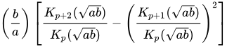
Variance	${\displaystyle \left({\frac {b}{a}}\right)\left[{\frac {K_{p+2}({\sqrt {ab}})}{K_{p}({\sqrt {ab}})}}-\left({\frac {K_{p+1}({\sqrt {ab}})}{K_{p}({\sqrt {ab}})}}\right)^{2}\right]}$
MGF	${\displaystyle \left({\frac {a}{a-2t}}\right)^{\frac {p}{2}}{\frac {K_{p}({\sqrt {b(a-2t)}})}{K_{p}({\sqrt {ab}})}}}$
CF	${\displaystyle \left({\frac {a}{a-2it}}\right)^{\frac {p}{2}}{\frac {K_{p}({\sqrt {b(a-2it)}})}{K_{p}({\sqrt {ab}})}}}$

In probability theory and statistics, the generalized inverse Gaussian distribution (GIG) is a three-parameter family of continuous probability distributions with probability density function

$${\displaystyle f(x)={\frac {(a/b)^{p/2}}{2K_{p}({\sqrt {ab}})}}x^{(p-1)}e^{-(ax+b/x)/2},\qquad x>0,}$$

where K_p is a modified Bessel function of the second kind, a > 0, b > 0 and p a real parameter. It is used extensively in geostatistics, statistical linguistics, finance, etc. This distribution was first proposed by Étienne Halphen.^[1][2][3] It was rediscovered and popularised by Ole Barndorff-Nielsen, who called it the generalized inverse Gaussian distribution. Its statistical properties are discussed in Bent Jørgensen's lecture notes.^[4]

By setting ${\displaystyle \theta ={\sqrt {ab}}}$ and ${\textstyle \eta ={\sqrt {b/a}}}$, we can alternatively express the GIG distribution as

$${\displaystyle f(x)={\frac {1}{2\eta K_{p}(\theta )}}\left({\frac {x}{\eta }}\right)^{p-1}e^{-\theta (x/\eta +\eta /x)/2},}$$

where ${\displaystyle \theta }$ is the concentration parameter while ${\displaystyle \eta }$ is the scaling parameter.

Barndorff-Nielsen and Halgreen proved that the GIG distribution is infinitely divisible.^[5]

The entropy of the generalized inverse Gaussian distribution is given as^{[citation needed]}

$${\displaystyle {\begin{aligned}H={\frac {1}{2}}\log \left({\frac {b}{a}}\right)&{}+\log \left(2K_{p}\left({\sqrt {ab}}\right)\right)-(p-1){\frac {\left[{\frac {d}{d\nu }}K_{\nu }\left({\sqrt {ab}}\right)\right]_{\nu =p}}{K_{p}\left({\sqrt {ab}}\right)}}\\&{}+{\frac {\sqrt {ab}}{2K_{p}\left({\sqrt {ab}}\right)}}\left(K_{p+1}\left({\sqrt {ab}}\right)+K_{p-1}\left({\sqrt {ab}}\right)\right)\end{aligned}}}$$

where ${\displaystyle \left[{\frac {d}{d\nu }}K_{\nu }\left({\sqrt {ab}}\right)\right]_{\nu =p}}$ is a derivative of the modified Bessel function of the second kind with respect to the order ${\displaystyle \nu }$ evaluated at ${\displaystyle \nu =p}$

The characteristic of a random variable ${\displaystyle X\sim GIG(p,a,b)}$ is given as^[4]

$${\displaystyle E(e^{itX})=\left({\frac {a}{a-2it}}\right)^{\frac {p}{2}}{\frac {K_{p}\left({\sqrt {(a-2it)b}}\right)}{K_{p}\left({\sqrt {ab}}\right)}}}$$

for ${\displaystyle t\in \mathbb {R} }$ where ${\displaystyle i}$ denotes the imaginary unit.

The inverse Gaussian and gamma distributions are special cases of the generalized inverse Gaussian distribution for p = −1/2 and b = 0, respectively.^[6] Specifically, an inverse Gaussian distribution of the form

$${\displaystyle f(x;\mu ,\lambda )=\left[{\frac {\lambda }{2\pi x^{3}}}\right]^{1/2}\exp {\left({\frac {-\lambda (x-\mu )^{2}}{2\mu ^{2}x}}\right)}}$$

is a GIG with ${\displaystyle a=\lambda /\mu ^{2}}$, ${\displaystyle b=\lambda }$, and ${\displaystyle p=-1/2}$. A gamma distribution of the form

$${\displaystyle g(x;\alpha ,\beta )=\beta ^{\alpha }{\frac {1}{\Gamma (\alpha )}}x^{\alpha -1}e^{-\beta x}}$$ is a GIG with ${\displaystyle a=2\beta }$, ${\displaystyle b=0}$, and ${\displaystyle p=\alpha }$.

Other special cases include the inverse-gamma distribution, for a = 0.^[6]

The GIG distribution is conjugate to the normal distribution when serving as the mixing distribution in a normal variance-mean mixture.^[7][8] Let the prior distribution for some hidden variable, say ${\displaystyle z}$, be GIG: $${\displaystyle P(z\mid a,b,p)=\operatorname {GIG} (z\mid a,b,p)}$$ and let there be ${\displaystyle T}$ observed data points, ${\displaystyle X=x_{1},\ldots ,x_{T}}$, with normal likelihood function, conditioned on ${\displaystyle z:}$

$${\displaystyle P(X\mid z,\alpha ,\beta )=\prod _{i=1}^{T}N(x_{i}\mid \alpha +\beta z,z)}$$

where ${\displaystyle N(x\mid \mu ,v)}$ is the normal distribution, with mean ${\displaystyle \mu }$ and variance ${\displaystyle v}$. Then the posterior for ${\displaystyle z}$, given the data is also GIG: $${\displaystyle P(z\mid X,a,b,p,\alpha ,\beta )={\text{GIG}}\left(z\mid a+T\beta ^{2},b+S,p-{\frac {T}{2}}\right)}$$ where ${\textstyle S=\sum _{i=1}^{T}(x_{i}-\alpha )^{2}}$.^{[note 1]}

The Sichel distribution results when the GIG is used as the mixing distribution for the Poisson parameter ${\displaystyle \lambda }$.^[9][10]

• Inverse Gaussian distribution
• Gamma distribution