Explore Black History

This article includes a list of general references but lacks sufficient corresponding inline citations. Please help improve this article by introducing more precise citations. (November 2024) (Learn how and when to remove this message)

In statistics and machine learning, Gaussian process approximation is a computational method that accelerates inference tasks in the context of a Gaussian process model, most commonly likelihood evaluation and prediction. Like approximations of other models, they can often be expressed as additional assumptions imposed on the model, which do not correspond to any actual feature, but which retain its key properties while simplifying calculations. Many of these approximation methods can be expressed in purely linear algebraic or functional analytic terms as matrix or function approximations. Others are purely algorithmic and cannot easily be rephrased as a modification of a statistical model.

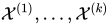
In statistical modeling, it is often convenient to assume that ${\displaystyle y\in {\mathcal {Y}}}$, the phenomenon under investigation is a Gaussian process indexed by ${\displaystyle X\in {\mathcal {X}}={\mathcal {X}}_{1}\times {\mathcal {X}}_{2}\dots {\mathcal {X}}_{d}}$ which has mean function ${\displaystyle \mu :{\mathcal {X}}\rightarrow {\mathcal {Y}}}$ and covariance function ${\displaystyle K:{\mathcal {X}}\times {\mathcal {X}}\rightarrow \mathbb {R} }$. One can also assume that data ${\displaystyle \mathbf {y} =(y_{1},\dots ,y_{n})}$ are values of a particular realization of this process for indices ${\displaystyle \mathbf {X} =X_{1},\dots ,X_{n}}$.

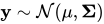
Consequently, the joint distribution of the data can be expressed as

${\displaystyle \mathbf {y} \sim {\mathcal {N}}(\mathbf {\mu } ,\mathbf {\Sigma } )}$,

where ${\displaystyle \mathbf {\Sigma } =\left[K(X_{i},X_{j})\right]_{i,j=1}^{n}}$ and ${\displaystyle \mathbf {\mu } =\left(\mu (X_{1}),\mu (X_{2}),\dots ,\mu (X_{d})\right)^{\top }}$, i.e. respectively a matrix with the covariance function values and a vector with the mean function values at corresponding (pairs of) indices. The negative log-likelihood of the data then takes the form

${\displaystyle -\log \ell (\mathbf {y} )={\frac {d}{2\pi }}+{\frac {1}{2}}\log \det(\mathbf {\Sigma } )+\left(\mathbf {y} -\mathbf {\mu } \right)^{\top }\mathbf {\Sigma } ^{-1}\left(\mathbf {y} -\mathbf {\mu } \right)}$

Similarly, the best predictor of ${\displaystyle \mathbf {y} ^{*}}$, the values of ${\displaystyle y}$ for indices ${\displaystyle \mathbf {X} ^{*}=\left(X_{1}^{*},X_{2}^{*},\dots ,X_{d}^{*}\right)}$, given data ${\displaystyle \mathbf {y} }$ has the form

${\displaystyle \mathbf {\mu } _{\mathbf {y} }^{*}=\mathbb {E} \left[\mathbf {y} ^{*}|\mathbf {y} \right]=\mathbf {\mu } ^{*}-\mathbf {\Sigma } _{\mathbf {y} ^{*}\mathbf {y} }\mathbf {\Sigma } ^{-1}\left(\mathbf {y} -\mathbf {\mu } \right)}$

In the context of Gaussian models, especially in geostatistics, prediction using the best predictor, i.e. mean conditional on the data, is also known as kriging.

The most computationally expensive component of the best predictor formula is inverting the covariance matrix ${\displaystyle \mathbf {\Sigma } }$, which has cubic complexity ${\displaystyle {\mathcal {O}}(n^{3})}$. Similarly, evaluating likelihood involves both calculating ${\displaystyle \mathbf {\Sigma } ^{-1}}$ and the determinant ${\displaystyle \det(\mathbf {\Sigma } )}$ which has the same cubic complexity.

Gaussian process approximations can often be expressed in terms of assumptions on ${\displaystyle y}$ under which ${\displaystyle \log \ell (\mathbf {y} )}$ and ${\displaystyle \mathbf {\mu } _{\mathbf {y} }^{*}}$ can be calculated with much lower complexity. Since these assumptions are generally not believed to reflect reality, the likelihood and the best predictor obtained in this way are not exact, but they are meant to be close to their original values.

This class of approximations is expressed through a set of assumptions which are imposed on the original process and which, typically, imply some special structure of the covariance matrix. Although most of these methods were developed independently, most of them can be expressed as special cases of the sparse general Vecchia approximation.

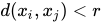
These methods approximate the true model in a way the covariance matrix is sparse. Typically, each method proposes its own algorithm that takes the full advantage of the sparsity pattern in the covariance matrix. Two prominent members of this class of approaches are covariance tapering and domain partitioning. The first method generally requires a metric ${\displaystyle d}$ over ${\displaystyle {\mathcal {X}}}$ and assumes that for ${\displaystyle X,{\tilde {X}}\in {\mathcal {X}}}$ we have ${\displaystyle Cov(y(X),y({\tilde {X}}))\neq 0}$ only if ${\displaystyle d(X,{\tilde {X}})<r}$ for some radius ${\displaystyle r}$. The second method assumes that there exist ${\displaystyle {\mathcal {X}}^{(1)},\dots ,{\mathcal {X}}^{(K)}}$ such that ${\displaystyle \bigcup _{k=1}^{K}{\mathcal {X}}^{(k)}}$. Then with appropriate distribution of indices among partition elements and ordering of elements of ${\displaystyle X}$ the covariance matrix is block diagonal.

This family of methods assumes that the precision matrix ${\displaystyle \mathbf {\Lambda } =\mathbf {\Sigma } ^{-1}}$ is sparse and generally specifies which of its elements are non-zero. This leads to fast inversion because only those elements need to be calculated. Some of the prominent approximations in this category include the approach based on the equivalence between Gaussian processes with Matern covariance function and stochastic PDEs, periodic embedding, and Nearest Neighbour Gaussian processes. The first method applies to the case of ${\displaystyle d=2}$ and when ${\displaystyle {\mathcal {X}}}$ has a defined metric and takes advantage of the fact, that the Markov property holds which makes ${\displaystyle \mathbf {\Lambda } }$ very sparse. The second extends the domain and uses Discrete Fourier Transform to decorrelate the data, which results in a diagonal precision matrix. The third one requires a metric on ${\displaystyle {\mathcal {X}}}$ and takes advantage of the so-called screening effect assuming that ${\displaystyle \mathbf {\Lambda } _{i,j}\neq 0}$ only if ${\displaystyle d(x_{i},x_{j})<r}$, for some ${\displaystyle r>0}$.

In many practical applications, calculating ${\displaystyle \mathbf {\Lambda } }$ is replaced with computing first ${\displaystyle \mathbf {L} }$, the Cholesky factor of ${\displaystyle \mathbf {\Sigma } }$, and second its inverse ${\displaystyle \mathbf {L} ^{-1}}$. This is known to be more stable than a plain inversion. For this reason, some authors focus on constructing a sparse approximation of the Cholesky factor of the precision or covariance matrices. One of the most established methods in this class is the Vecchia approximation and its generalization. These approaches determine the optimal ordering of indices and, consequently, the elements of ${\displaystyle \mathbf {x} }$ and then assume a dependency structure which minimizes in-fill in the Cholesky factor. Several other methods can be expressed in this framework, the Multi-resolution Approximation (MRA) and Nearest Neighbour Gaussian Process.

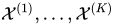
While this approach encompasses many methods, the common assumption underlying them all is the assumption, that ${\displaystyle y}$, the Gaussian process of interest, is effectively low-rank. More precisely, it is assumed, that there exists a set of indices ${\displaystyle {\bar {X}}=\{{\bar {x}}_{1},\dots ,{\bar {x}}_{p}\}}$ such that every other set of indices ${\displaystyle X=\{x_{1},\dots ,x_{n}\}}$

${\displaystyle y(X)\sim {\mathcal {N}}\left(\mathbf {A} _{X}{\bar {\mathbf {\mu } }},\mathbf {A} _{X}^{\top }{\bar {\mathbf {\Sigma } }}\mathbf {A} _{X}+\mathbf {D} \right)}$

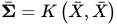
where ${\displaystyle \mathbf {A} _{X}}$ is an ${\displaystyle p\times k}$ matrix, ${\displaystyle {\bar {\mathbf {\mu } }}=\mu \left(y\left({\bar {X}}\right)\right)}$ and ${\displaystyle {\bar {\mathbf {\Sigma } }}=K\left({\bar {X}},{\bar {X}}\right)}$ and ${\displaystyle \mathbf {D} }$ is a diagonal matrix. Depending on the method and application various ways of selecting ${\displaystyle {\bar {X}}}$ have been proposed. Typically, ${\displaystyle p}$ is selected to be much smaller than ${\displaystyle n}$ which means that the computational cost of inverting ${\displaystyle {\bar {\mathbf {\Sigma } }}}$ is manageable (${\displaystyle {\mathcal {O}}(p^{3})}$ instead of ${\displaystyle {\mathcal {O}}(n^{3})}$).

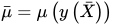
More generally, on top of selecting ${\displaystyle {\bar {X}}}$, one may also find an ${\displaystyle n\times p}$ matrix ${\displaystyle \mathbf {A} }$ and assume that ${\displaystyle X=\mathbf {A} \mathbf {\eta } }$, where ${\displaystyle \mathbf {\eta } }$ are ${\displaystyle p}$ values of a Gaussian process possibly independent of ${\displaystyle x}$. Many machine learning methods fall into this category, such as subset-of-regressors (SoR), relevance vector machine, sparse spectrum Gaussian Process and others and they generally differ in the way they derive ${\displaystyle \mathbf {A} }$ and ${\displaystyle \mathbf {\eta } }$.

A full-scale approximation combines a low-rank approximation, typically based on inducing points, with an approximation of the residual process. The low-rank component captures global or large-scale dependence, while the residual approximation recovers local and fine-scale dependence that is not adequately represented by the low-rank component. Different variants obtain computational sparsity by applying methods such as covariance tapering to the residual covariance matrix or a Vecchia approximation to the residual process.^[1][2]

The general principle of hierarchical approximations consists of a repeated application of some other method, such that each consecutive application refines the quality of the approximation. Even though they can be expressed as a set of statistical assumptions, they are often described in terms of a hierarchical matrix approximation (HODLR) or basis function expansion (LatticeKrig, MRA, wavelets). The hierarchical matrix approach can often be represented as a repeated application of a low-rank approximation to successively smaller subsets of the index set ${\displaystyle X}$. Basis function expansion relies on using functions with compact support. These features can then be exploited by an algorithm who steps through consecutive layers of the approximation. In the most favourable settings some of these methods can achieve quasi-linear (${\displaystyle {\mathcal {O}}(n\log n)}$) complexity.

Probabilistic graphical models provide a convenient framework for comparing model-based approximations. In this context, value of the process at index ${\displaystyle x_{k}\in X}$ can then be represented by a vertex in a directed graph and edges correspond to the terms in the factorization of the joint density of ${\displaystyle y(X)}$. In general, when no independent relations are assumed, the joint probability distribution can be represented by an arbitrary directed acyclic graph. Using a particular approximation can then be expressed as a certain way of ordering the vertices and adding or removing specific edges.

This class of methods does not specify a statistical model or impose assumptions on an existing one. Three major members of this group are the meta-kriging algorithm, the gapfill algorithm and Local Approximate Gaussian Process approach. The first one partitions the set of indices into ${\displaystyle K}$ components ${\displaystyle {\mathcal {X}}^{(1)},\dots ,{\mathcal {X}}^{(k)}}$, calculates the conditional distribution for each those components separately and then uses geometric median of the conditional PDFs to combine them. The second is based on quantile regression using values of the process which are close to the value one is trying to predict, where distance is measured in terms of a metric on the set of indices. Local Approximate Gaussian Process uses a similar logic but constructs a valid stochastic process based on these neighboring values.

• Liu, Haitao; Ong, Yew-Soon; Shen, Xiaobo; Cai, Jianfei (2020). "When Gaussian Process Meets Big Data: A Review of Scalable GPS". IEEE Transactions on Neural Networks and Learning Systems. PP (11): 1–19. arXiv:1807.01065. doi:10.1109/TNNLS.2019.2957109. PMID 31944966.
• Heaton, Matthew J.; Datta, Abhirup and Pavan s/o Leosesuraja; Finley, Andrew O.; Furrer, Reinhard; Guinness, Joseph; Guhaniyogi, Rajarshi; Gerber, Florian; Gramacy, Robert B.; Hammerling, Dorit; Katzfuss, Matthias; Lindgren, Finn; Nychka, Douglas W.; Sun, Furong; Zammit-Mangion, Andrew (2018). "A Case Study Competition Among Methods for Analyzing Large Spatial Data". Journal of Agricultural, Biological and Environmental Statistics. 24 (3): 398–425. doi:10.1007/s13253-018-00348-w. ISSN 1085-7117. PMC 6709111. PMID 31496633.
• Banerjee, Sudipto (2017). "High-Dimensional Bayesian Geostatistics". Bayesian Analysis. 12 (2): 583–614. doi:10.1214/17-BA1056R. PMC 5790125. PMID 29391920.