Explore Black History

In the statistical theory of estimation, the German tank problem consists of estimating the maximum of a discrete uniform distribution from sampling without replacement. In simple terms, suppose there exists an unknown number of items which are sequentially numbered from 1 to N. A random sample of these items is taken and their sequence numbers observed; the problem is to estimate N from these observed numbers.

The problem can be approached using either frequentist inference or Bayesian inference, leading to different results. Estimating the population maximum based on a single sample yields divergent results, whereas estimation based on multiple samples is a practical estimation question whose answer is simple (especially in the frequentist setting) but not obvious (especially in the Bayesian setting).

The problem is named after its historical application by Allied forces in World War II to estimate the monthly rate of German tank production from very limited data. The statistical method exploited the manufacturing practice of assigning and attaching ascending serial-number sequences to tank components (chassis, gearbox, engine, wheels), with some of the tanks eventually captured in battle by Allied forces. This contrasted with conventional intelligence, which often overestimated Nazi output; this statistical approach yielded a highly accurate estimate.^[1]

The adversary is presumed to have manufactured a series of tanks marked with consecutive whole numbers, beginning with serial number 1. Additionally, regardless of a tank's date of manufacture, history of service, or the serial number it bears, the distribution over serial numbers becoming revealed to analysis is uniform, up to the point in time when the analysis is conducted.

Assuming tanks are assigned sequential serial numbers starting with 1, suppose that four tanks are captured and that they have the serial numbers: 19, 40, 42 and 60.

A frequentist approach (using the minimum-variance unbiased estimator) predicts the total number of tanks produced will be:

${\displaystyle N\approx 74}$

A Bayesian approach (using a uniform prior over the integers in ${\displaystyle [4,\Omega ]}$ for any suitably large ${\displaystyle \Omega }$) predicts that the median number of tanks produced will be very similar to the frequentist prediction:

${\displaystyle N_{med}\approx 73.9}$

whereas the Bayesian mean predicts that the number of tanks produced would be:

${\displaystyle N_{av}\approx 89}$

Let N equal the total number of tanks predicted to have been produced, m equal the highest serial number observed and k equal the number of tanks captured.

The frequentist prediction is calculated as:

${\displaystyle N\approx m+{\frac {m}{k}}-1=74}$

The Bayesian median is calculated as:

${\displaystyle N_{med}\approx m+{\frac {m\ln(2)}{k-1}}=73.9}$

The Bayesian mean is calculated as:

${\displaystyle N_{av}\approx (m-1){\frac {k-1}{k-2}}=89}$

These Bayesian quantities are derived from the Bayesian posterior distribution:

${\displaystyle \Pr(N=n)={\begin{cases}0&{\text{if }}n<m,\\{\frac {k-1}{k}}{\frac {\binom {m-1}{k-1}}{\binom {n}{k}}}&{\text{if }}n\geq m.\end{cases}}}$

This probability mass function has a positive skewness, related to the fact that there are at least 60 tanks. Because of this skewness, the mean may not be the most meaningful estimate. The median in this example is 74.5, in close agreement with the frequentist formula. Using Stirling's approximation, the posterior may be approximated by an exponentially decaying function of n,

${\displaystyle \Pr(N=n)\approx {\begin{cases}0&{\text{if }}n<m\\(k-1)m^{k-1}n^{-k}&{\text{if }}n\geq m,\end{cases}}}$

which results in the following approximation for the median:

${\displaystyle N_{med}\approx m+{\frac {m\ln(2)}{k-1}}}$

and the following approximations for the mean and standard deviation:

${\displaystyle {\begin{aligned}N&\approx \mu \pm \sigma =89\pm 50,\\[5pt]\mu &=(m-1){\frac {k-1}{k-2}},\\[5pt]\sigma &={\sqrt {\frac {(k-1)(m-1)(m-k+1)}{(k-3)(k-2)^{2}}}}.\end{aligned}}}$

During the course of the Second World War, the Western Allies made sustained efforts to determine the extent of German production and approached this in two major ways: conventional intelligence gathering and statistical estimation. In many cases, statistical analysis substantially improved on conventional intelligence. In some cases, conventional intelligence was used in conjunction with statistical methods, as was the case in estimation of Panther tank production just prior to D-Day.

The allied command structure had thought the Panzer V (Panther) tanks seen in Italy, with their high velocity, long-barreled 75 mm/L70 guns, were unusual heavy tanks and would only be seen in northern France in small numbers, much the same way as the Tiger I was seen in Tunisia. The US Army was confident that the Sherman tank would continue to perform well, as it had versus the Panzer III and Panzer IV tanks in North Africa and Sicily.^[a] Shortly before D-Day, rumors indicated that large numbers of Panzer V tanks were being used.

To determine whether this was true, the Allies attempted to estimate the number of tanks being produced. To do this, they used the serial numbers on captured or destroyed tanks. The principal numbers used were gearbox numbers, as these fell in two unbroken sequences. Chassis and engine numbers were also used, though their use was more complicated. Various other components were used to cross-check the analysis. Similar analyses were done on wheels, which were observed to be sequentially numbered (i.e., 1, 2, 3, ..., N).^[3][b][4][5]

The analysis of tank wheels yielded an estimate for the number of wheel molds that were in use. A discussion with British road wheel makers then estimated the number of wheels that could be produced from this many molds, which yielded the number of tanks that were being produced each month. Analysis of wheels from two tanks (32 road wheels each, 64 road wheels total) yielded an estimate of 270 tanks produced in February 1944, substantially more than had previously been suspected.^[6]

German records after the war showed production for the month of February 1944 was 276.^[7][c] The statistical approach proved to be far more accurate than conventional intelligence methods, and the phrase "German tank problem" became accepted as a descriptor for this type of statistical analysis.

Estimating production was not the only use of this serial-number analysis. It was also used to understand German production more generally, including number of factories, relative importance of factories, length of supply chain (based on lag between production and use), changes in production, and use of resources such as rubber.

According to conventional Allied intelligence estimates, the Germans were producing around 1,400 tanks a month between June 1940 and September 1942. Applying the formula below to the serial numbers of captured tanks, the number was calculated to be 246 a month. After the war, captured German production figures from the ministry of Albert Speer showed the actual number to be 245.^[4]

Estimates for some specific months are given as:^[8]

Similar serial-number analysis was used for other military equipment during World War II, most successfully for the V-2 rocket.^[9]

Factory markings on Soviet military equipment were analyzed during the Korean War, and by German intelligence during World War II.^[10]

In the 1980s, some Americans were given access to the production line of Israel's Merkava tanks. The production numbers were classified, but the tanks had serial numbers, allowing estimation of production.^[11]

The formula has been used in non-military contexts, for example to estimate the number of Commodore 64 computers built, where the result (12.5 million) matches the low-end estimates.^[12]

This section does not cite any sources. Please help improve this section by adding citations to reliable sources. Unsourced material may be challenged and removed. (January 2013) (Learn how and when to remove this message)

To confound serial-number analysis, serial numbers can be excluded, or usable auxiliary information reduced. Alternatively, serial numbers that resist cryptanalysis can be used, most effectively by randomly choosing numbers without replacement from a list that is much larger than the number of objects produced, or by producing random numbers and checking them against the list of already assigned numbers; collisions are likely to occur unless the number of digits possible is more than twice the number of digits in the number of objects produced; this is valid for serial numbers in any base (see: Birthday problem).^[d] For this, a cryptographically secure pseudorandom number generator may be used. All these methods require a lookup table (or breaking the cypher) to back out from serial number to production order, which complicates use of serial numbers: a range of serial numbers cannot be recalled, for instance, but each must be looked up individually, or a list generated.

Alternatively, sequential serial numbers can be encrypted with a simple substitution cipher, which allows easy decoding, but is also easily broken by frequency analysis: even if starting from an arbitrary point, the plaintext has a pattern (namely, numbers are in sequence). One example is given in Ken Follett's novel Code to Zero, where the encryption of the Jupiter-C rocket serial numbers is given by:

The code word here is Huntsville (with repeated letters omitted) to get a 10-letter key.^[13] The rocket number 13 was therefore "HN", and the rocket number 24 was "UT".

For point estimation (estimating a single value for the total, ${\displaystyle {\widehat {N}}}$), the minimum-variance unbiased estimator (MVUE, or UMVU estimator) is given by:^[e]

${\displaystyle {\widehat {N}}=m(1+k^{-1})-1,}$

where m is the largest serial number observed (sample maximum) and k is the number of tanks observed (sample size).^[11][14] Note that once a serial number has been observed, it is no longer in the pool and will not be observed again.

This has a variance^[11]

${\displaystyle \operatorname {var} \left({\widehat {N}}\right)={\frac {1}{k}}{\frac {(N-k)(N+1)}{(k+2)}}\approx {\frac {N^{2}}{k^{2}}}{\text{ for small samples }}k\ll N,}$

so the standard deviation is approximately N/k, the expected size of the gap between sorted observations in the sample.

The formula may be understood intuitively as the sample maximum plus the average gap between observations in the sample, the sample maximum being chosen as the initial estimator, due to being the maximum likelihood estimator,^[f] with the gap being added to compensate for the negative bias of the sample maximum as an estimator for the population maximum,^[g] and written as

${\displaystyle {\widehat {N}}=m+{\frac {m-k}{k}}=m+mk^{-1}-1=m(1+k^{-1})-1.}$

This can be visualized by imagining that the observations in the sample are evenly spaced throughout the range, with additional observations just outside the range at 0 and N + 1. If starting with an initial gap between 0 and the lowest observation in the sample (the sample minimum), the average gap between consecutive observations in the sample is ${\displaystyle (m-k)/k}$, the ${\displaystyle -k}$ being because the observations themselves are not counted in computing the gap between observations.^[h] A derivation of the expected value and the variance of the sample maximum are shown in the page of the discrete uniform distribution.

This philosophy is formalized and generalized in the method of maximum spacing estimation; a similar heuristic is used for plotting position in a Q–Q plot, plotting sample points at k / (n + 1), which is evenly on the uniform distribution, with a gap at the end.

Instead of, or in addition to, point estimation, interval estimation can be carried out, such as confidence intervals. These are easily computed, based on the observation that the probability that k observations in the sample will fall in an interval covering p of the range (0 ≤ p ≤ 1) is p^k (assuming in this section that draws are with replacement, to simplify computations; if draws are without replacement, this overstates the likelihood, and intervals will be overly conservative).

Thus the sampling distribution of the quantile of the sample maximum is the graph x^1/k from 0 to 1: the p-th to q-th quantile of the sample maximum m are the interval [p^1/kN, q^1/kN]. Inverting this yields the corresponding confidence interval for the population maximum of [m/q^1/k, m/p^1/k].

For example, taking the symmetric 95% interval p = 2.5% and q = 97.5% for k = 5 yields 0.025^1/5 ≈ 0.48, 0.975^1/5 ≈ 0.995, so the confidence interval is approximately [1.005m, 2.08m]. The lower bound is very close to m, thus more informative is the asymmetric confidence interval from p = 5% to 100%; for k = 5 this yields 0.05^1/5 ≈ 0.55 and the interval [m, 1.82m].

More generally, the (downward biased) 95% confidence interval is [m, m/0.05^1/k] = [m, m·20^1/k]. For a range of k values, with the UMVU point estimator (plus 1 for legibility) for reference, this yields:

Immediate observations are:

• For small sample sizes, the confidence interval is very wide, reflecting great uncertainty in the estimate.
• The range shrinks rapidly, reflecting the exponentially decaying probability that all observations in the sample will be significantly below the maximum.
• The confidence interval exhibits positive skew, as N can never be below the sample maximum, but can potentially be arbitrarily high above it.

Note that m/k cannot be used naively (or rather (m + m/k − 1)/k) as an estimate of the standard error SE, as the standard error of an estimator is based on the population maximum (a parameter), and using an estimate to estimate the error in that very estimate is circular reasoning.

The Bayesian approach to the German tank problem^[15] is to consider the posterior probability ${\displaystyle (N=n\mid M=m,K=k)}$ that the number of enemy tanks ${\displaystyle N}$ is ${\displaystyle n}$, when the number of observed tanks ${\displaystyle K}$ is ${\displaystyle k}$, and the maximum observed serial number ${\displaystyle M}$ is ${\displaystyle m}$. Note that this does not discard the relevant information contained in the samples, as we will see that the likelihood function can be constructed using only the number of samples and the max observed value.

The answer to this problem depends on the choice of prior for ${\displaystyle N}$. One can proceed using a proper prior over the positive integers, e.g., the Poisson or Negative Binomial distribution, where a closed formula for the posterior mean and posterior variance can be obtained.^[16] Below, we will instead adopt a bounded uniform prior.

For brevity, in what follows, ${\displaystyle (N=n\mid M=m,K=k)}$ is written ${\displaystyle (n\mid m,k)}$.

The rule for conditional probability gives

${\displaystyle (n\mid m,k)(m\mid k)=(m\mid n,k)(n\mid k)=(m,n\mid k)}$

The expression

${\displaystyle (m\mid n,k)=(M=m\mid N=n,K=k)}$

is the conditional probability that the maximum serial number observed, ${\displaystyle M}$, is equal to ${\displaystyle m}$, when the number of enemy tanks, ${\displaystyle N}$, is known to be equal to ${\displaystyle n}$, and the number of enemy tanks observed, ${\displaystyle K}$, is known to be equal to ${\displaystyle k}$.

It is

${\displaystyle (m\mid n,k)={\binom {m-1}{k-1}}{\binom {n}{k}}^{-1}[k\leq m][m\leq n]}$

where ${\displaystyle {\binom {n}{k}}}$ is a binomial coefficient and ${\displaystyle [k\leq n]}$ is an Iverson bracket.

The expression can be derived as follows: ${\displaystyle (m\mid n,k)}$ answers the question: "What is the probability of a specific serial number ${\displaystyle m}$ being the highest number observed in a sample of ${\displaystyle k}$ tanks, given there are ${\displaystyle n}$ tanks in total?"

One can think of the sample of size ${\displaystyle k}$ to be the result of ${\displaystyle k}$ individual draws without replacement. Assume ${\displaystyle m}$ is observed on draw number ${\displaystyle d}$. The probability of this occurring is: $${\displaystyle \underbrace {{\frac {m-1}{n}}\cdot {\frac {m-2}{n-1}}\cdot {\frac {m-3}{n-2}}\cdots {\frac {m-d+1}{n-d+2}}} _{d-1{\text{ times}}}\cdot \underbrace {\frac {1}{n-d+1}} _{{\text{draw no. }}d}\cdot \underbrace {{\frac {m-d}{n-d}}\cdot {\frac {m-d-1}{n-d-1}}\cdots {\frac {m-d-(k-d-1)}{n-d-(k-d-1)}}} _{k-d{\text{ times}}}={\frac {(n-k)!}{n!}}\cdot {\frac {(m-1)!}{(m-k)!}}.}$$

As can be seen from the right-hand side, this expression is independent of ${\displaystyle d}$ and therefore the same for each ${\displaystyle d\leq k}$. As ${\displaystyle m}$ can be drawn on ${\displaystyle k}$ different draws, the probability of any specific ${\displaystyle m}$ being the largest one observed is ${\displaystyle k}$ times the above probability: $${\displaystyle (m\mid n,k)=k\cdot {\frac {(n-k)!}{n!}}\cdot {\frac {(m-1)!}{(m-k)!}}={\binom {m-1}{k-1}}{\binom {n}{k}}^{-1}.}$$

Seen differently, after ${\displaystyle k}$ draws without replacement, one draw was for object ${\displaystyle m}$, and the other ${\displaystyle k-1}$ were for objects in the range ${\displaystyle 1}$ to ${\displaystyle m-1}$ ; there are ${\displaystyle {\binom {m-1}{k-1}}}$ ways to achieve this. And there are ${\displaystyle {\binom {n}{k}}}$ ways to draw without replacement ${\displaystyle k}$ objects from a collection of ${\displaystyle n}$ objects.

The expression ${\displaystyle (m\mid k)=(M=m\mid K=k)}$ is the probability that the maximum serial number is equal to ${\displaystyle m}$ once ${\displaystyle k}$ tanks have been observed but before the serial numbers have actually been observed.

The expression ${\displaystyle (m\mid k)}$ can be re-written in terms of the other quantities by marginalizing over all possible ${\displaystyle n}$.

${\displaystyle {\begin{aligned}(m\mid k)&=\sum _{n=0}^{\infty }(m,n\mid k)\\&=\sum _{n=0}^{\infty }(m\mid n,k)(n\mid k)\end{aligned}}}$

We assume that ${\displaystyle k}$ is fixed in advance so that we do not have to consider any distribution over ${\displaystyle k}$. Thus, our prior can depend on ${\displaystyle k}$.

The expression

${\displaystyle (n\mid k)=(N=n\mid K=k)}$

is the credibility that the total number of tanks, ${\displaystyle N}$, is equal to ${\displaystyle n}$ when the number ${\displaystyle K}$ tanks observed is known to be ${\displaystyle k}$, but before the serial numbers have been observed. Assume that it is some discrete uniform distribution

${\displaystyle (n\mid k)=(\Omega -k)^{-1}[k\leq n][n<\Omega ]}$

The upper limit ${\displaystyle \Omega }$ must be finite, because the function

${\displaystyle f(n)=\lim _{\Omega \rightarrow \infty }(\Omega -k)^{-1}[k\leq n][n<\Omega ]=0}$

is not a mass distribution function. Our result below will not depend on ${\displaystyle \Omega }$.

Provided that ${\displaystyle \Omega >m}$, so that the prior is consistent with the observed data:

${\displaystyle (n\mid m,k)=(m\mid n,k)\left(\sum _{n=m}^{\Omega -1}(m\mid n,k)\right)^{-1}[m\leq n][n<\Omega ]}$

As ${\displaystyle \Omega \rightarrow \infty }$, the summation approaches ${\displaystyle \sum _{n=m}^{\infty }(m\mid n,k)}$ (which is finite if k ≥ 2). Thus, for suitably large ${\displaystyle \Omega }$, we have

${\displaystyle (n\mid m,k)\approx (m\mid n,k)\left(\sum _{n=m}^{\infty }(m\mid n,k)\right)^{-1}[m\leq n]}$

For k ≥ 1 the mode of the distribution of the number of enemy tanks is m.

For k ≥ 2, the credibility that the number of enemy tanks is equal to ${\displaystyle n}$, is

${\displaystyle (N=n\mid m,k)=(k-1){\binom {m-1}{k-1}}k^{-1}{\binom {n}{k}}^{-1}[m\leq n]}$

The credibility that the number of enemy tanks, N, is greater than n, is

${\displaystyle (N>n\mid m,k)={\begin{cases}1&{\text{if }}n<m\\{\frac {\binom {m-1}{k-1}}{\binom {n}{k-1}}}&{\text{if }}n\geq m\end{cases}}}$

For k ≥ 3, N has the finite mean value:

${\displaystyle (m-1)(k-1)(k-2)^{-1}}$

For k ≥ 4, N has the finite standard deviation:

${\displaystyle (k-1)^{1/2}(k-2)^{-1}(k-3)^{-1/2}(m-1)^{1/2}(m+1-k)^{1/2}}$

These formulas are derived below.

The following binomial coefficient identity is used below for simplifying series relating to the German Tank Problem.

${\displaystyle \sum _{n=m}^{\infty }{\frac {1}{\binom {n}{k}}}={\frac {k}{k-1}}{\frac {1}{\binom {m-1}{k-1}}}}$

This sum formula is somewhat analogous to the integral formula

${\displaystyle \int _{n=m}^{\infty }{\frac {dn}{n^{k}}}={\frac {1}{k-1}}{\frac {1}{m^{k-1}}}}$

These formulas apply for k > 1.

Observing one tank randomly out of a population of n tanks gives the serial number m with probability 1/n for m ≤ n, and zero probability for m > n. Using Iverson bracket notation this is written

${\displaystyle (M=m\mid N=n,K=1)=(m\mid n)={\frac {[m\leq n]}{n}}}$

This is the conditional probability mass distribution function of ${\displaystyle m}$.

When considered a function of n for fixed m this is a likelihood function.

${\displaystyle {\mathcal {L}}(n)={\frac {[n\geq m]}{n}}}$

The maximum likelihood estimate for the total number of tanks is N₀ = m, clearly a biased estimate since the true number can be more than this, potentially many more, but cannot be fewer.

The marginal likelihood (i.e. marginalized over all models) is infinite, being a tail of the harmonic series.

${\displaystyle \sum _{n}{\mathcal {L}}(n)=\sum _{n=m}^{\infty }{\frac {1}{n}}=\infty }$

but

${\displaystyle {\begin{aligned}\sum _{n}{\mathcal {L}}(n)[n<\Omega ]&=\sum _{n=m}^{\Omega -1}{\frac {1}{n}}\\[5pt]&=H_{\Omega -1}-H_{m-1}\end{aligned}}}$

where ${\displaystyle H_{n}}$ is the harmonic number.

The credibility mass distribution function depends on the prior limit ${\displaystyle \Omega }$:

${\displaystyle {\begin{aligned}&(N=n\mid M=m,K=1)\\[5pt]={}&(n\mid m)={\frac {[m\leq n]}{n}}{\frac {[n<\Omega ]}{H_{\Omega -1}-H_{m-1}}}\end{aligned}}}$

The mean value of ${\displaystyle N}$ is

${\displaystyle {\begin{aligned}\sum _{n}n\cdot (n\mid m)&=\sum _{n=m}^{\Omega -1}{\frac {1}{H_{\Omega -1}-H_{m-1}}}\\[5pt]&={\frac {\Omega -m}{H_{\Omega -1}-H_{m-1}}}\\[5pt]&\approx {\frac {\Omega -m}{\log \left({\frac {\Omega -1}{m-1}}\right)}}\end{aligned}}}$

If two tanks rather than one are observed, then the probability that the larger of the observed two serial numbers is equal to m, is

${\displaystyle (M=m\mid N=n,K=2)=(m\mid n)=[m\leq n]{\frac {m-1}{\binom {n}{2}}}}$

When considered a function of n for fixed m this is a likelihood function

${\displaystyle {\mathcal {L}}(n)=[n\geq m]{\frac {m-1}{\binom {n}{2}}}}$

The total likelihood is

${\displaystyle {\begin{aligned}\sum _{n}{\mathcal {L}}(n)&={\frac {m-1}{1}}\sum _{n=m}^{\infty }{\frac {1}{\binom {n}{2}}}\\[4pt]&={\frac {m-1}{1}}\cdot {\frac {2}{2-1}}\cdot {\frac {1}{\binom {m-1}{2-1}}}\\[4pt]&=2\end{aligned}}}$

and the credibility mass distribution function is

${\displaystyle {\begin{aligned}&(N=n\mid M=m,K=2)\\[4pt]={}&(n\mid m)\\[4pt]={}&{\frac {{\mathcal {L}}(n)}{\sum _{n}{\mathcal {L}}(n)}}\\[4pt]={}&[n\geq m]{\frac {m-1}{n(n-1)}}\end{aligned}}}$

The median ${\displaystyle {\tilde {N}}}$ satisfies

${\displaystyle \sum _{n}[n\geq {\tilde {N}}](n\mid m)={\frac {1}{2}}}$

so

${\displaystyle {\frac {m-1}{{\tilde {N}}-1}}={\frac {1}{2}}}$

and so the median is

${\displaystyle {\tilde {N}}=2m-1}$

but the mean value of ${\displaystyle N}$ is infinite

${\displaystyle \mu =\sum _{n}n\cdot (n\mid m)={\frac {m-1}{1}}\sum _{n=m}^{\infty }{\frac {1}{n-1}}=\infty }$

The conditional probability that the largest of k observations taken from the serial numbers {1,...,n}, is equal to m, is

${\displaystyle {\begin{aligned}&(M=m\mid N=n,K=k\geq 2)\\={}&(m\mid n,k)\\={}&[m\leq n]{\frac {\binom {m-1}{k-1}}{\binom {n}{k}}}\end{aligned}}}$

The likelihood function of n is the same expression

${\displaystyle {\mathcal {L}}(n)=[n\geq m]{\frac {\binom {m-1}{k-1}}{\binom {n}{k}}}}$

The total likelihood is finite for k ≥ 2:

${\displaystyle {\begin{aligned}\sum _{n}{\mathcal {L}}(n)&={\frac {\binom {m-1}{k-1}}{1}}\sum _{n=m}^{\infty }{1 \over {\binom {n}{k}}}\\&={\frac {\binom {m-1}{k-1}}{1}}\cdot {\frac {k}{k-1}}\cdot {\frac {1}{\binom {m-1}{k-1}}}\\&={\frac {k}{k-1}}\end{aligned}}}$

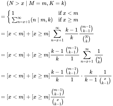
The credibility mass distribution function is

${\displaystyle {\begin{aligned}&(N=n\mid M=m,K=k\geq 2)=(n\mid m,k)\\={}&{\frac {{\mathcal {L}}(n)}{\sum _{n}{\mathcal {L}}(n)}}\\={}&[n\geq m]{\frac {k-1}{k}}{\frac {\binom {m-1}{k-1}}{\binom {n}{k}}}\\={}&[n\geq m]{\frac {m-1}{n}}{\frac {\binom {m-2}{k-2}}{\binom {n-1}{k-1}}}\\={}&[n\geq m]{\frac {m-1}{n}}{\frac {m-2}{n-1}}{\frac {k-1}{k-2}}{\frac {\binom {m-3}{k-3}}{\binom {n-2}{k-2}}}\end{aligned}}}$

The complementary cumulative distribution function is the credibility that N > x

${\displaystyle {\begin{aligned}&(N>x\mid M=m,K=k)\\[4pt]={}&{\begin{cases}1&{\text{if }}x<m\\\sum _{n=x+1}^{\infty }(n\mid m,k)&{\text{if }}x\geq m\end{cases}}\\={}&[x<m]+[x\geq m]\sum _{n=x+1}^{\infty }{\frac {k-1}{k}}{\frac {\binom {m-1}{k-1}}{\binom {N}{k}}}\\[4pt]={}&[x<m]+[x\geq m]{\frac {k-1}{k}}{\frac {\binom {m-1}{k-1}}{1}}\sum _{n=x+1}^{\infty }{\frac {1}{\binom {n}{k}}}\\[4pt]={}&[x<m]+[x\geq m]{\frac {k-1}{k}}{\frac {\binom {m-1}{k-1}}{1}}\cdot {\frac {k}{k-1}}{\frac {1}{\binom {x}{k-1}}}\\[4pt]={}&[x<m]+[x\geq m]{\frac {\binom {m-1}{k-1}}{\binom {x}{k-1}}}\end{aligned}}}$

The cumulative distribution function is the credibility that N ≤ x

${\displaystyle {\begin{aligned}&(N\leq x\mid M=m,K=k)\\[4pt]={}&1-(N>x\mid M=m,K=k)\\[4pt]={}&[x\geq m]\left(1-{\frac {\binom {m-1}{k-1}}{\binom {x}{k-1}}}\right)\end{aligned}}}$

The order of magnitude of the number of enemy tanks is

${\displaystyle {\begin{aligned}\mu &=\sum _{n}n\cdot (N=n\mid M=m,K=k)\\[4pt]&=\sum _{n}n[n\geq m]{\frac {m-1}{n}}{\frac {\binom {m-2}{k-2}}{\binom {n-1}{k-1}}}\\[4pt]&={\frac {m-1}{1}}{\frac {\binom {m-2}{k-2}}{1}}\sum _{n=m}^{\infty }{\frac {1}{\binom {n-1}{k-1}}}\\[4pt]&={\frac {m-1}{1}}{\frac {\binom {m-2}{k-2}}{1}}\cdot {\frac {k-1}{k-2}}{\frac {1}{\binom {m-2}{k-2}}}\\[4pt]&={\frac {m-1}{1}}{\frac {k-1}{k-2}}\end{aligned}}}$

The statistical uncertainty is the standard deviation ${\displaystyle \sigma }$, satisfying the equation

${\displaystyle \sigma ^{2}+\mu ^{2}=\sum _{n}n^{2}\cdot (N=n\mid M=m,K=k)}$

So

${\displaystyle {\begin{aligned}\sigma ^{2}+\mu ^{2}-\mu &=\sum _{n}n(n-1)\cdot (N=n\mid M=m,K=k)\\[4pt]&=\sum _{n=m}^{\infty }n(n-1){\frac {m-1}{n}}{\frac {m-2}{n-1}}{\frac {k-1}{k-2}}{\frac {\binom {m-3}{k-3}}{\binom {n-2}{k-2}}}\\[4pt]&={\frac {m-1}{1}}{\frac {m-2}{1}}{\frac {k-1}{k-2}}\cdot {\frac {\binom {m-3}{k-3}}{1}}\sum _{n=m}^{\infty }{\frac {1}{\binom {n-2}{k-2}}}\\[4pt]&={\frac {m-1}{1}}{\frac {m-2}{1}}{\frac {k-1}{k-2}}{\frac {\binom {m-3}{k-3}}{1}}{\frac {k-2}{k-3}}{\frac {1}{\binom {m-3}{k-3}}}\\[4pt]&={\frac {m-1}{1}}{\frac {m-2}{1}}{\frac {k-1}{k-3}}\end{aligned}}}$

and

${\displaystyle {\begin{aligned}\sigma &={\sqrt {{\frac {m-1}{1}}{\frac {m-2}{1}}{\frac {k-1}{k-3}}+\mu -\mu ^{2}}}\\[4pt]&={\sqrt {\frac {(k-1)(m-1)(m-k+1)}{(k-3)(k-2)^{2}}}}\end{aligned}}}$

The variance-to-mean ratio is simply

${\displaystyle {\frac {\sigma ^{2}}{\mu }}={\frac {m-k+1}{(k-3)(k-2)}}}$

• Mark and recapture, other method of estimating population size
• Maximum spacing estimation, which generalizes the intuition of "assume uniformly distributed"
• Copernican principle and Lindy effect, analogous predictions of lifetime assuming just one observation in the sample (current age).
  • The Doomsday argument, application to estimate expected survival time of the human race.
• Generalized extreme value distribution, possible limit distributions of sample maximum (opposite question).
• Maximum likelihood
• Bias of an estimator
• Likelihood function

• Goodman, L. A. (1954). "Some Practical Techniques in Serial Number Analysis". Journal of the American Statistical Association. 49 (265). American Statistical Association: 97–112. doi:10.2307/2281038. JSTOR 2281038.

• Grime, James (31 July 2024). "The Clever Way to Count Tanks - Numberphile" (video). YouTube. Brady Haran. Retrieved 18 October 2024.