Explore Black History

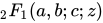
In mathematics, the Gaussian or ordinary hypergeometric function ₂F₁(a, b; c; z) is a special function represented by the hypergeometric series, that includes many other special functions as specific or limiting cases. It is a solution of a second-order linear ordinary differential equation (ODE). Every second-order linear ODE with three regular singular points can be transformed into this equation.

For systematic lists of some of the many thousands of published identities involving the hypergeometric function, see the reference works by Erdélyi et al. (1953) and Olde Daalhuis (2010). There is no known system for organizing all of the identities; indeed, there is no known algorithm that can generate all identities; a number of different algorithms are known that generate different series of identities. The theory of the algorithmic discovery of identities remains an active research topic.

The term "hypergeometric series" was first used by John Wallis in his 1655 book Arithmetica Infinitorum.

Hypergeometric series were studied by Leonhard Euler, but the first full systematic treatment was given by Carl Friedrich Gauss (1813).

Studies in the nineteenth century included those of Ernst Kummer (1836), and the fundamental characterisation by Bernhard Riemann (1857) of the hypergeometric function by means of the differential equation it satisfies.

Riemann showed that the second-order differential equation for ₂F₁(z), examined in the complex plane, could be characterised (on the Riemann sphere) by its three regular singularities.

The cases where the solutions are algebraic functions were found by Hermann Schwarz (Schwarz's list).

The hypergeometric function is defined for |z| < 1 by the power series

$${\displaystyle {}_{2}F_{1}(a,b;c;z)=\sum _{n=0}^{\infty }{\frac {(a)_{n}(b)_{n}}{(c)_{n}}}{\frac {z^{n}}{n!}}=1+{\frac {ab}{c}}{\frac {z}{1!}}+{\frac {a(a+1)b(b+1)}{c(c+1)}}{\frac {z^{2}}{2!}}+\cdots .}$$

It is undefined (or infinite) if c equals a non-positive integer. Here (q)_n is the (rising) Pochhammer symbol,^{[note 1]} which is defined by:

$${\displaystyle (q)_{n}={\begin{cases}1&n=0\\q(q+1)\cdots (q+n-1)&n>0\end{cases}}}$$

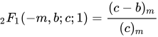
The series terminates if either a or b is a nonpositive integer, in which case the function reduces to a polynomial:

$${\displaystyle {}_{2}F_{1}(-m,b;c;z)=\sum _{n=0}^{m}(-1)^{n}{\binom {m}{n}}{\frac {(b)_{n}}{(c)_{n}}}z^{n}.}$$

For complex arguments z with |z| ≥ 1 it can be analytically continued along any path in the complex plane that avoids the branch points 1 and infinity. In practice, most computer implementations of the hypergeometric function adopt a branch cut along the line z ≥ 1.

As c → −m, where m is a non-negative integer, one has ₂F₁(z) → ∞. Dividing by the value Γ(c) of the gamma function, we have the limit:

$${\displaystyle \lim _{c\to -m}{\frac {{}_{2}F_{1}(a,b;c;z)}{\Gamma (c)}}={\frac {(a)_{m+1}(b)_{m+1}}{(m+1)!}}z^{m+1}{}_{2}F_{1}(a+m+1,b+m+1;m+2;z)}$$

₂F₁(z) is the most common type of generalized hypergeometric series _pF_q.

Using the identity ${\displaystyle (a)_{n+1}=a(a+1)_{n}}$, it is shown that

$${\displaystyle {\frac {d}{dz}}\ {}_{2}F_{1}(a,b;c;z)={\frac {ab}{c}}\ {}_{2}F_{1}(a+1,b+1;c+1;z)}$$

and more generally,

$${\displaystyle {\frac {d^{n}}{dz^{n}}}\ {}_{2}F_{1}(a,b;c;z)={\frac {(a)_{n}(b)_{n}}{(c)_{n}}}\ {}_{2}F_{1}(a+n,b+n;c+n;z)}$$

Many of the common mathematical functions can be expressed in terms of the hypergeometric function, or as limiting cases of it. Some typical examples are

$${\displaystyle {\begin{aligned}_{2}F_{1}\left(1,1;2;-z\right)&={\frac {\ln(1+z)}{z}}\\_{2}F_{1}(a,b;b;z)&=(1-z)^{-a}\quad (b{\text{ arbitrary}})\\_{2}F_{1}\left({\frac {1}{2}},{\frac {1}{2}};{\frac {3}{2}};z^{2}\right)&={\frac {\arcsin(z)}{z}}\\\,_{2}F_{1}\left({\frac {1}{3}},{\frac {2}{3}};{\frac {3}{2}};-{\frac {27x^{2}}{4}}\right)&={\frac {{\sqrt[{3}]{\frac {3x{\sqrt {3}}+{\sqrt {27x^{2}+4}}}{2}}}-{\sqrt[{3}]{\frac {2}{3x{\sqrt {3}}+{\sqrt {27x^{2}+4}}}}}}{x{\sqrt {3}}}}\end{aligned}}}$$ When a = 1 and b = c, the series reduces into a plain geometric series, i.e. $${\displaystyle {\begin{aligned}_{2}F_{1}\left(1,b;b;z\right)&={_{1}F_{0}}\left(1;;z\right)=1+z+z^{2}+z^{3}+z^{4}+\cdots \end{aligned}}}$$

hence, the name hypergeometric. This function can be considered as a generalization of the geometric series.

The confluent hypergeometric function (or Kummer's function) can be given as a limit of the hypergeometric function

$${\displaystyle M(a,c,z)=\lim _{b\to 0}{_{2}F_{1}}(a,b^{-1};c;bz)}$$

so all functions that are essentially special cases of it, such as Bessel functions, can be expressed as limits of hypergeometric functions. These include most of the commonly used functions of mathematical physics.

Legendre functions are solutions of a second order differential equation with 3 regular singular points so can be expressed in terms of the hypergeometric function in many ways, for example

$${\displaystyle {}_{2}F_{1}(a,1-a;c;z)=\Gamma (c)z^{\tfrac {1-c}{2}}(1-z)^{\tfrac {c-1}{2}}P_{-a}^{1-c}(1-2z)}$$

Several orthogonal polynomials, including Jacobi polynomials P^(α,β)
_n and their special cases Legendre polynomials, Chebyshev polynomials, Gegenbauer polynomials, Zernike polynomials can be written in terms of hypergeometric functions using

$${\displaystyle {}_{2}F_{1}(-n,\alpha +1+\beta +n;\alpha +1;x)={\frac {n!}{(\alpha +1)_{n}}}P_{n}^{(\alpha ,\beta )}(1-2x)}$$

Other polynomials that are special cases include Krawtchouk polynomials, Meixner polynomials, Meixner–Pollaczek polynomials.

Given ${\displaystyle z\in \mathbb {C} \setminus \{0,1\}}$, let

$${\displaystyle \tau ={\rm {i}}{\frac {{}_{2}F_{1}{\bigl (}{\frac {1}{2}},{\frac {1}{2}};1;1-z{\bigr )}}{{}_{2}F_{1}{\bigl (}{\frac {1}{2}},{\frac {1}{2}};1;z{\bigr )}}}.}$$

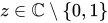
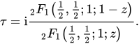
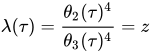
Then

$${\displaystyle \lambda (\tau )={\frac {\theta _{2}(\tau )^{4}}{\theta _{3}(\tau )^{4}}}=z}$$

is the modular lambda function, where

$${\displaystyle \theta _{2}(\tau )=\sum _{n\in \mathbb {Z} }e^{\pi i\tau (n+1/2)^{2}},\quad \theta _{3}(\tau )=\sum _{n\in \mathbb {Z} }e^{\pi i\tau n^{2}}.}$$

The j-invariant, a modular function, is a rational function in ${\displaystyle \lambda (\tau )}$.

Incomplete beta functions B_x(p, q) are related by

$${\displaystyle B_{x}(p,q)={\tfrac {x^{p}}{p}}{}_{2}F_{1}(p,1-q;p+1;x).}$$

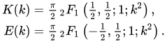
The complete elliptic integrals K and E are given by^[1]

$${\displaystyle {\begin{aligned}K(k)&={\tfrac {\pi }{2}}\,_{2}F_{1}\left({\tfrac {1}{2}},{\tfrac {1}{2}};1;k^{2}\right),\\E(k)&={\tfrac {\pi }{2}}\,_{2}F_{1}\left(-{\tfrac {1}{2}},{\tfrac {1}{2}};1;k^{2}\right).\end{aligned}}}$$

The hypergeometric function is a solution of Euler's hypergeometric differential equation

$${\displaystyle z(1-z){\frac {d^{2}w}{dz^{2}}}+\left[c-(a+b+1)z\right]{\frac {dw}{dz}}-ab\,w=0.}$$

which has three regular singular points: 0,1 and ∞. The generalization of this equation to three arbitrary regular singular points is given by Riemann's differential equation. Any second order linear differential equation with three regular singular points can be converted to the hypergeometric differential equation by a change of variables.

Solutions to the hypergeometric differential equation are built out of the hypergeometric series ₂F₁(a, b; c; z). The equation has two linearly independent solutions. At each of the three singular points 0, 1, ∞, there are usually two special solutions of the form x^s times a holomorphic function of x, where s is one of the two roots of the indicial equation and x is a local variable vanishing at a regular singular point. This gives 3 × 2 = 6 special solutions, as follows.

Around the point z = 0, two independent solutions are, if c is not a non-positive integer,

$${\displaystyle _{2}F_{1}(a,b;c;z)}$$

and, on condition that c is not an integer,

$${\displaystyle z^{1-c}{_{2}F_{1}}(1+a-c,1+b-c;2-c;z)}$$

If c is a non-positive integer 1 − m, then the first of these solutions does not exist and must be replaced by ${\displaystyle z^{m}F(a+m,b+m;1+m;z).}$ The second solution does not exist when c is an integer greater than 1, and is equal to the first solution, or its replacement, when c is any other integer. So when c is an integer, a more complicated expression must be used for a second solution, equal to the first solution multiplied by ln(z), plus another series in powers of z, involving the digamma function. See Olde Daalhuis (2010) for details.

Around z = 1, if c − a − b is not an integer, one has two independent solutions

$${\displaystyle \,_{2}F_{1}(a,b;1+a+b-c;1-z)}$$

and

$${\displaystyle (1-z)^{c-a-b}\;_{2}F_{1}(c-a,c-b;1+c-a-b;1-z)}$$

Around z = ∞, if a − b is not an integer, one has two independent solutions

$${\displaystyle z^{-a}\,_{2}F_{1}\left(a,1+a-c;1+a-b;z^{-1}\right)}$$

and

$${\displaystyle z^{-b}\,_{2}F_{1}\left(b,1+b-c;1+b-a;z^{-1}\right).}$$

Again, when the conditions of non-integrality are not met, there exist other solutions that are more complicated.

Any 3 of the above 6 solutions satisfy a linear relation as the space of solutions is 2-dimensional, giving (⁶
₃) = 20 linear relations between them called connection formulas.

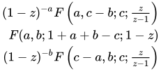
A second order Fuchsian equation with n singular points has a group of symmetries acting (projectively) on its solutions, isomorphic to the Coxeter group W(D_n) of order 2ⁿ⁻¹n!. The hypergeometric equation is the case n = 3, with group of order 24 isomorphic to the symmetric group on 4 points, as first described by Kummer. The appearance of the symmetric group is accidental and has no analogue for more than 3 singular points, and it is sometimes better to think of the group as an extension of the symmetric group on 3 points (acting as permutations of the 3 singular points) by a Klein 4-group (whose elements change the signs of the differences of the exponents at an even number of singular points). Kummer's group of 24 transformations is generated by the three transformations taking a solution F(a, b; c; z) to one of

$${\displaystyle {\begin{aligned}(1-z)^{-a}F\left(a,c-b;c;{\tfrac {z}{z-1}}\right)\\F(a,b;1+a+b-c;1-z)\\(1-z)^{-b}F\left(c-a,b;c;{\tfrac {z}{z-1}}\right)\end{aligned}}}$$

which correspond to the transpositions (12), (23), and (34) under an isomorphism with the symmetric group on 4 points 1, 2, 3, 4. (The first and third of these are actually equal to F(a, b; c; z) whereas the second is an independent solution to the differential equation.)

Applying Kummer's 24 = 6×4 transformations to the hypergeometric function gives the 6 = 2×3 solutions above corresponding to each of the 2 possible exponents at each of the 3 singular points, each of which appears 4 times because of the identities

$${\displaystyle {\begin{aligned}{}_{2}F_{1}(a,b;c;z)&=(1-z)^{c-a-b}\,{}_{2}F_{1}(c-a,c-b;c;z)&&{\text{Euler transformation}}\\{}_{2}F_{1}(a,b;c;z)&=(1-z)^{-a}\,{}_{2}F_{1}(a,c-b;c;{\tfrac {z}{z-1}})&&{\text{Pfaff transformation}}\\{}_{2}F_{1}(a,b;c;z)&=(1-z)^{-b}\,{}_{2}F_{1}(c-a,b;c;{\tfrac {z}{z-1}})&&{\text{Pfaff transformation}}\end{aligned}}}$$

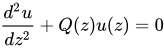
The hypergeometric differential equation may be brought into the Q-form

$${\displaystyle {\frac {d^{2}u}{dz^{2}}}+Q(z)u(z)=0}$$

by making the substitution u = wv and eliminating the first-derivative term. One finds that

$${\displaystyle Q={\frac {z^{2}[1-(a-b)^{2}]+z[2c(a+b-1)-4ab]+c(2-c)}{4z^{2}(1-z)^{2}}}}$$

and v is given by the solution to

$${\displaystyle {\frac {d}{dz}}\log v(z)=-{\frac {c-z(a+b+1)}{2z(1-z)}}=-{\frac {c}{2z}}-{\frac {1+a+b-c}{2(z-1)}}}$$

which is

$${\displaystyle v(z)=z^{-c/2}(1-z)^{(c-a-b-1)/2}.}$$

The Q-form is significant in its relation to the Schwarzian derivative (Hille 1976, pp. 307–401).

The Schwarz triangle maps or Schwarz s-functions are ratios of pairs of solutions.

$${\displaystyle s_{k}(z)={\frac {\phi _{k}^{(1)}(z)}{\phi _{k}^{(0)}(z)}}}$$

where k is one of the points 0, 1, ∞. The notation

$${\displaystyle D_{k}(\lambda ,\mu ,\nu ;z)=s_{k}(z)}$$

is also sometimes used. Note that the connection coefficients become Möbius transformations on the triangle maps.

Note that each triangle map is regular at z ∈ {0, 1, ∞} respectively, with

$${\displaystyle {\begin{aligned}s_{0}(z)&=z^{\lambda }(1+{\mathcal {O}}(z))\\s_{1}(z)&=(1-z)^{\mu }(1+{\mathcal {O}}(1-z))\end{aligned}}}$$ and $${\displaystyle s_{\infty }(z)=z^{\nu }(1+{\mathcal {O}}({\tfrac {1}{z}})).}$$

In the special case of λ, μ and ν real, with 0 ≤ λ,μ,ν < 1 then the s-maps are conformal maps of the upper half-plane H to triangles on the Riemann sphere, bounded by circular arcs. This mapping is a generalization of the Schwarz–Christoffel mapping to triangles with circular arcs. The singular points 0,1 and ∞ are sent to the triangle vertices. The angles of the triangle are πλ, πμ and πν respectively.

Furthermore, in the case of λ=1/p, μ=1/q and ν=1/r for integers p, q, r, then the triangle tiles the sphere, the complex plane or the upper half plane according to whether λ + μ + ν − 1 is positive, zero or negative; and the s-maps are inverse functions of automorphic functions for the triangle group 〈p, q, r〉 = Δ(p, q, r).

The monodromy of a hypergeometric equation describes how fundamental solutions change when analytically continued around paths in the z plane that return to the same point. That is, when the path winds around a singularity of ₂F₁, the value of the solutions at the endpoint will differ from the starting point.

Two fundamental solutions of the hypergeometric equation are related to each other by a linear transformation; thus the monodromy is a mapping (group homomorphism):

$${\displaystyle \pi _{1}(\mathbf {C} \setminus \{0,1\},z_{0})\to {\text{GL}}(2,\mathbf {C} )}$$

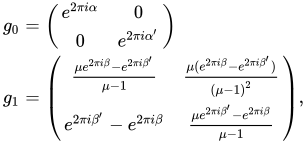
where π₁ is the fundamental group. In other words, the monodromy is a two dimensional linear representation of the fundamental group. The monodromy group of the equation is the image of this map, i.e. the group generated by the monodromy matrices. The monodromy representation of the fundamental group can be computed explicitly in terms of the exponents at the singular points.^[2] If (α, α'), (β, β') and (γ,γ') are the exponents at 0, 1 and ∞, then, taking z₀ near 0, the loops around 0 and 1 have monodromy matrices

$${\displaystyle {\begin{aligned}g_{0}&={\begin{pmatrix}e^{2\pi i\alpha }&0\\0&e^{2\pi i\alpha ^{\prime }}\end{pmatrix}}\\g_{1}&={\begin{pmatrix}{\mu e^{2\pi i\beta }-e^{2\pi i\beta ^{\prime }} \over \mu -1}&{\mu (e^{2\pi i\beta }-e^{2\pi i\beta ^{\prime }}) \over (\mu -1)^{2}}\\e^{2\pi i\beta ^{\prime }}-e^{2\pi i\beta }&{\mu e^{2\pi i\beta ^{\prime }}-e^{2\pi i\beta } \over \mu -1}\end{pmatrix}},\end{aligned}}}$$

where

$${\displaystyle \mu ={\sin \pi (\alpha +\beta ^{\prime }+\gamma ^{\prime })\sin \pi (\alpha ^{\prime }+\beta +\gamma ^{\prime }) \over \sin \pi (\alpha ^{\prime }+\beta ^{\prime }+\gamma ^{\prime })\sin \pi (\alpha +\beta +\gamma ^{\prime })}.}$$

If 1 − a, c − a − b, a − b are non-integer rational numbers with denominators k, l, m then the monodromy group is finite if and only if ${\displaystyle 1/k+1/l+1/m>1}$, see Schwarz's list or Kovacic's algorithm.

If B is the beta function then

$${\displaystyle \mathrm {B} (b,c-b){_{2}F_{1}}(a,b;c;z)=\int _{0}^{1}x^{b-1}(1-x)^{c-b-1}(1-zx)^{-a}\,dx\qquad \Re (c)>\Re (b)>0,}$$

provided that z is not a real number such that it is greater than or equal to 1. This can be proved by expanding (1 − zx)^−a using the binomial theorem and then integrating term by term for z with absolute value smaller than 1, and by analytic continuation elsewhere. When z is a real number greater than or equal to 1, analytic continuation must be used, because (1 − zx) is zero at some point in the support of the integral, so the value of the integral may be ill-defined. This was given by Euler in 1748 and implies Euler's and Pfaff's hypergeometric transformations.

Other representations, corresponding to other branches, are given by taking the same integrand, but taking the path of integration to be a closed Pochhammer cycle enclosing the singularities in various orders. Such paths correspond to the monodromy action.

Barnes used the theory of residues to evaluate the Barnes integral

$${\displaystyle {\frac {1}{2\pi i}}\int _{-i\infty }^{i\infty }{\frac {\Gamma (a+s)\Gamma (b+s)\Gamma (-s)}{\Gamma (c+s)}}(-z)^{s}\,ds}$$

as

$${\displaystyle {\frac {\Gamma (a)\Gamma (b)}{\Gamma (c)}}\,_{2}F_{1}(a,b;c;z),}$$

where the contour is drawn to separate the poles 0, 1, 2... from the poles −a, −a − 1, ..., −b, −b − 1, ... . This is valid as long as z is not a nonnegative real number.

The Gauss hypergeometric function can be written as a John transform (Gelfand, Gindikin & Graev 2003, 2.1.2).

The six functions

$${\displaystyle {}_{2}F_{1}(a\pm 1,b;c;z),\quad {}_{2}F_{1}(a,b\pm 1;c;z),\quad {}_{2}F_{1}(a,b;c\pm 1;z)}$$

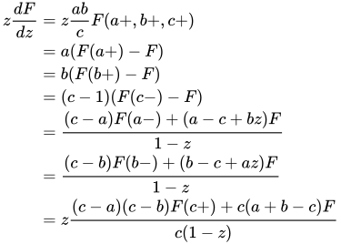
are called contiguous to ₂F₁(a, b; c; z). Gauss showed that ₂F₁(a, b; c; z) can be written as a linear combination of any two of its contiguous functions, with rational coefficients in terms of a, b, c, and z. This gives

$${\displaystyle {\begin{pmatrix}6\\2\end{pmatrix}}=15}$$

relations, given by identifying any two lines on the right hand side of

$${\displaystyle {\begin{aligned}z{\frac {dF}{dz}}&=z{\frac {ab}{c}}F(a+,b+,c+)\\&=a(F(a+)-F)\\&=b(F(b+)-F)\\&=(c-1)(F(c-)-F)\\&={\frac {(c-a)F(a-)+(a-c+bz)F}{1-z}}\\&={\frac {(c-b)F(b-)+(b-c+az)F}{1-z}}\\&=z{\frac {(c-a)(c-b)F(c+)+c(a+b-c)F}{c(1-z)}}\end{aligned}}}$$

where F = ₂F₁(a, b; c; z), F(a+) = ₂F₁(a + 1, b; c; z), and so on. Repeatedly applying these relations gives a linear relation over C(z) between any three functions of the form

$${\displaystyle {_{2}F_{1}}(a+m,b+n;c+l;z),}$$

where m, n, and l are integers.^{[3] [4]}

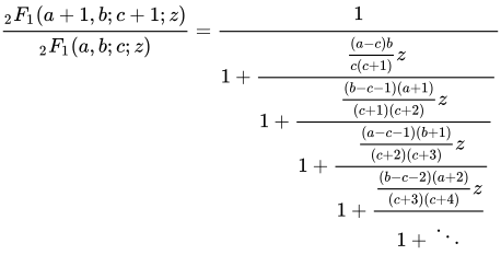
Gauss used the contiguous relations to give several ways to write a quotient of two hypergeometric functions as a continued fraction, for example:

$${\displaystyle {\frac {{}_{2}F_{1}(a+1,b;c+1;z)}{{}_{2}F_{1}(a,b;c;z)}}={\cfrac {1}{1+{\cfrac {{\frac {(a-c)b}{c(c+1)}}z}{1+{\cfrac {{\frac {(b-c-1)(a+1)}{(c+1)(c+2)}}z}{1+{\cfrac {{\frac {(a-c-1)(b+1)}{(c+2)(c+3)}}z}{1+{\cfrac {{\frac {(b-c-2)(a+2)}{(c+3)(c+4)}}z}{1+{}\ddots }}}}}}}}}}}$$

Transformation formulas relate two hypergeometric functions at different values of the argument z.

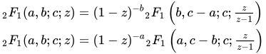
Euler's transformation is $${\displaystyle {}_{2}F_{1}(a,b;c;z)=(1-z)^{c-a-b}{}_{2}F_{1}(c-a,c-b;c;z).}$$ It follows by combining the two Pfaff transformations $${\displaystyle {\begin{aligned}{}_{2}F_{1}(a,b;c;z)&=(1-z)^{-b}{}_{2}F_{1}\left(b,c-a;c;{\tfrac {z}{z-1}}\right)\\{}_{2}F_{1}(a,b;c;z)&=(1-z)^{-a}{}_{2}F_{1}\left(a,c-b;c;{\tfrac {z}{z-1}}\right)\\\end{aligned}}}$$ which in turn follow from Euler's integral representation. For extension of Euler's first and second transformations, see Rathie & Paris (2007) and Rakha & Rathie (2011). It can also be written as linear combination $${\displaystyle {\begin{aligned}{}_{2}F_{1}(a,b;c;z)={}&{\frac {\Gamma (c)\Gamma (c-a-b)}{\Gamma (c-a)\Gamma (c-b)}}{}_{2}F_{1}(a,b;a+b+1-c;1-z)\\[6pt]&{}+{\frac {\Gamma (c)\Gamma (a+b-c)}{\Gamma (a)\Gamma (b)}}(1-z)^{c-a-b}{}_{2}F_{1}(c-a,c-b;1+c-a-b;1-z).\end{aligned}}}$$

If two of the numbers 1 − c, c − 1, a − b, b − a, a + b − c, c − a − b are equal or one of them is 1/2 then there is a quadratic transformation of the hypergeometric function, connecting it to a different value of z related by a quadratic equation. The first examples were given by Kummer (1836), and a complete list was given by Goursat (1881). A typical example is

$${\displaystyle {}_{2}F_{1}(a,b;2b;z)=(1-z)^{-{\frac {a}{2}}}{}_{2}F_{1}\left({\tfrac {1}{2}}a,b-{\tfrac {1}{2}}a;b+{\tfrac {1}{2}};{\frac {z^{2}}{4z-4}}\right)}$$

If 1−c, a−b, a+b−c differ by signs or two of them are 1/3 or −1/3 then there is a cubic transformation of the hypergeometric function, connecting it to a different value of z related by a cubic equation. The first examples were given by Goursat (1881). A typical example is

$${\displaystyle {}_{2}F_{1}\left({\tfrac {3}{2}}a,{\tfrac {1}{2}}(3a-1);a+{\tfrac {1}{2}};-{\tfrac {z^{2}}{3}}\right)=(1+z)^{1-3a}\,{}_{2}F_{1}\left(a-{\tfrac {1}{3}},a;2a;2z(3+z^{2})(1+z)^{-3}\right)}$$

There are also some transformations of degree 4 and 6. Transformations of other degrees only exist if a, b, and c are certain rational numbers (Vidunas 2005). For example, $${\displaystyle {}_{2}F_{1}\left({\tfrac {1}{4}},{\tfrac {3}{8}};{\tfrac {7}{8}};z\right)(z^{4}-60z^{3}+134z^{2}-60z+1)^{1/16}={}_{2}F_{1}\left({\tfrac {1}{48}},{\tfrac {17}{48}};{\tfrac {7}{8}};{\tfrac {-432z(z-1)^{2}(z+1)^{8}}{(z^{4}-60z^{3}+134z^{2}-60z+1)^{3}}}\right).}$$

See Slater (1966, Appendix III) for a list of summation formulas at special points, most of which also appear in Bailey (1935). Gessel & Stanton (1982) gives further evaluations at more points. Koepf (1995) shows how most of these identities can be verified by computer algorithms.

Gauss's summation theorem, named for Carl Friedrich Gauss, is the identity

$${\displaystyle {}_{2}F_{1}(a,b;c;1)={\frac {\Gamma (c)\Gamma (c-a-b)}{\Gamma (c-a)\Gamma (c-b)}},\qquad \Re (c)>\Re (a+b)}$$

which follows from Euler's integral formula by putting z = 1. It includes the Vandermonde identity as a special case.

For the special case where ${\displaystyle a=-m}$, $${\displaystyle {}_{2}F_{1}(-m,b;c;1)={\frac {(c-b)_{m}}{(c)_{m}}}}$$

Dougall's formula generalizes this to the bilateral hypergeometric series at z = 1.

There are many cases where hypergeometric functions can be evaluated at z = −1 by using a quadratic transformation to change z = −1 to z = 1 and then using Gauss's theorem to evaluate the result. A typical example is Kummer's theorem, named for Ernst Kummer:

$${\displaystyle {}_{2}F_{1}(a,b;1+a-b;-1)={\frac {\Gamma (1+a-b)\Gamma (1+{\tfrac {1}{2}}a)}{\Gamma (1+a)\Gamma (1+{\tfrac {1}{2}}a-b)}}}$$

which follows from Kummer's quadratic transformations

$${\displaystyle {\begin{aligned}_{2}F_{1}(a,b;1+a-b;z)&=(1-z)^{-a}\;_{2}F_{1}\left({\frac {a}{2}},{\frac {1+a}{2}}-b;1+a-b;-{\frac {4z}{(1-z)^{2}}}\right)\\&=(1+z)^{-a}\,_{2}F_{1}\left({\frac {a}{2}},{\frac {a+1}{2}};1+a-b;{\frac {4z}{(1+z)^{2}}}\right)\end{aligned}}}$$

and Gauss's theorem by putting z = −1 in the first identity. For generalization of Kummer's summation, see Lavoie, Grondin & Rathie (1996).

Gauss's second summation theorem is

$${\displaystyle _{2}F_{1}\left(a,b;{\tfrac {1}{2}}\left(1+a+b\right);{\tfrac {1}{2}}\right)={\frac {\Gamma ({\tfrac {1}{2}})\Gamma ({\tfrac {1}{2}}\left(1+a+b\right))}{\Gamma ({\tfrac {1}{2}}\left(1+a)\right)\Gamma ({\tfrac {1}{2}}\left(1+b\right))}}.}$$

Bailey's theorem is

$${\displaystyle _{2}F_{1}\left(a,1-a;c;{\tfrac {1}{2}}\right)={\frac {\Gamma ({\tfrac {1}{2}}c)\Gamma ({\tfrac {1}{2}}\left(1+c\right))}{\Gamma ({\tfrac {1}{2}}\left(c+a\right))\Gamma ({\tfrac {1}{2}}\left(1+c-a\right))}}.}$$

For generalizations of Gauss's second summation theorem and Bailey's summation theorem, see Lavoie, Grondin & Rathie (1996).

There are many other formulas giving the hypergeometric function as an algebraic number at special rational values of the parameters, some of which are listed in Gessel & Stanton (1982) and Koepf (1995). Some typical examples are given by

$${\displaystyle {}_{2}F_{1}\left(a,-a;{\tfrac {1}{2}};{\tfrac {x^{2}}{4(x-1)}}\right)={\frac {(1-x)^{a}+(1-x)^{-a}}{2}},}$$

which can be restated as

$${\displaystyle T_{a}(\cos x)={}_{2}F_{1}\left(a,-a;{\tfrac {1}{2}};{\tfrac {1}{2}}(1-\cos x)\right)=\cos(ax)}$$

whenever −π < x < π and T is the (generalized) Chebyshev polynomial.

• Appell series
• Basic hypergeometric series
• Bilateral hypergeometric series
• Elliptic hypergeometric series
• General hypergeometric function
• Generalized hypergeometric series
• Hypergeometric distribution
• Lauricella hypergeometric series
• Modular hypergeometric series
• Riemann's differential equation

• "Hypergeometric function", Encyclopedia of Mathematics, EMS Press, 2001 [1994]
• John Pearson, Computation of Hypergeometric Functions (University of Oxford, MSc Thesis)
• Marko Petkovsek, Herbert Wilf and Doron Zeilberger, The book "A = B" (freely downloadable)
• Weisstein, Eric W. "Hypergeometric Function". MathWorld.