Explore Black History

In mathematics, the kernel of a linear map, also known as the null space or nullspace, is the part of the domain which is mapped to the zero vector of the co-domain; the kernel is always a linear subspace of the domain.^[1] That is, given a linear map L : V → W between two vector spaces V and W, the kernel of L is the vector space of all elements v of V such that L(v) = 0, where 0 denotes the zero vector in W,^[2] or more symbolically: $${\displaystyle \ker(L)=\left\{\mathbf {v} \in V\mid L(\mathbf {v} )=\mathbf {0} \right\}=L^{-1}(\mathbf {0} ).}$$

The kernel of L is a linear subspace of the domain V.^[3][2]

In the linear map ${\displaystyle L:V\to W,}$ two elements of V have the same image in W if and only if their difference lies in the kernel of L, that is,

$${\displaystyle L\left(\mathbf {v} _{1}\right)=L\left(\mathbf {v} _{2}\right)\quad \iff \quad L\left(\mathbf {v} _{1}-\mathbf {v} _{2}\right)=\mathbf {0} .}$$

From this, it follows by the first isomorphism theorem that the image of L is isomorphic to the quotient of V by the kernel: $${\displaystyle \operatorname {im} (L)\cong V/\ker(L).}$$ In the case where V is finite-dimensional, this implies the rank–nullity theorem: $${\displaystyle \dim(\ker L)+\dim(\operatorname {im} L)=\dim(V).}$$ where the term rank refers to the dimension of the image of L, ${\displaystyle \dim(\operatorname {im} L),}$ while nullity refers to the dimension of the kernel of L, ${\displaystyle \dim(\ker L).}$^[4] That is, $${\displaystyle \operatorname {Rank} (L)=\dim(\operatorname {im} L)\qquad {\text{ and }}\qquad \operatorname {Nullity} (L)=\dim(\ker L),}$$ so that the rank–nullity theorem can be restated as $${\displaystyle \operatorname {Rank} (L)+\operatorname {Nullity} (L)=\dim \left(\operatorname {domain} L\right).}$$

When V is an inner product space, the quotient ${\displaystyle V/\ker(L)}$ can be identified with the orthogonal complement in V of ${\displaystyle \ker(L)}$. This is the generalization to linear operators of the row space, or coimage, of a matrix.

The notion of kernel also makes sense for homomorphisms of modules, which are generalizations of vector spaces where the scalars are elements of a ring, rather than a field. The domain of the mapping is a module, with the kernel constituting a submodule. Here, the concepts of rank and nullity do not necessarily apply.

If V and W are topological vector spaces such that W is finite-dimensional, then a linear operator L: V → W is continuous if and only if the kernel of L is a closed subspace of V.

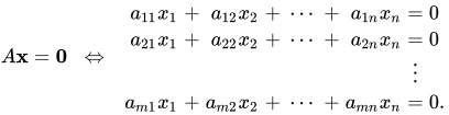
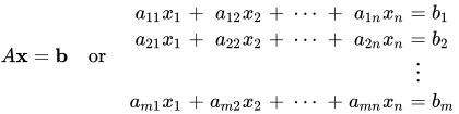
Consider a linear map represented as a m × n matrix A with coefficients in a field K (typically ${\displaystyle \mathbb {R} }$ or ${\displaystyle \mathbb {C} }$), that is operating on column vectors x with n components over K. The kernel of this linear map is the set of solutions to the equation Ax = 0, where 0 is understood as the zero vector. The dimension of the kernel of A is called the nullity of A. In set-builder notation, $${\displaystyle \operatorname {N} (A)=\operatorname {Null} (A)=\operatorname {ker} (A)=\left\{\mathbf {x} \in K^{n}\mid A\mathbf {x} =\mathbf {0} \right\}.}$$ The matrix equation is equivalent to a homogeneous system of linear equations: $${\displaystyle A\mathbf {x} =\mathbf {0} \;\;\Leftrightarrow \;\;{\begin{alignedat}{7}a_{11}x_{1}&&\;+\;&&a_{12}x_{2}&&\;+\;\cdots \;+\;&&a_{1n}x_{n}&&\;=\;&&&0\\a_{21}x_{1}&&\;+\;&&a_{22}x_{2}&&\;+\;\cdots \;+\;&&a_{2n}x_{n}&&\;=\;&&&0\\&&&&&&&&&&\vdots \ \;&&&\\a_{m1}x_{1}&&\;+\;&&a_{m2}x_{2}&&\;+\;\cdots \;+\;&&a_{mn}x_{n}&&\;=\;&&&0{\text{.}}\\\end{alignedat}}}$$ Thus the kernel of A is the same as the solution set to the above homogeneous equations.

The kernel of a m × n matrix A over a field K is a linear subspace of Kⁿ. That is, the kernel of A, the set Null(A), has the following three properties:

1. Null(A) always contains the zero vector, since A0 = 0.
2. If x ∈ Null(A) and y ∈ Null(A), then x + y ∈ Null(A). This follows from the distributivity of matrix multiplication over addition.
3. If x ∈ Null(A) and c is a scalar c ∈ K, then cx ∈ Null(A), since A(cx) = c(Ax) = c0 = 0.

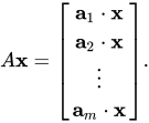
The product Ax can be written in terms of the dot product of vectors as follows: $${\displaystyle A\mathbf {x} ={\begin{bmatrix}\mathbf {a} _{1}\cdot \mathbf {x} \\\mathbf {a} _{2}\cdot \mathbf {x} \\\vdots \\\mathbf {a} _{m}\cdot \mathbf {x} \end{bmatrix}}.}$$

Here, a₁, ... , a_m denote the rows of the matrix A. It follows that x is in the kernel of A, if and only if x is orthogonal (or perpendicular) to each of the row vectors of A (since orthogonality is defined as having a dot product of 0).

The row space, or coimage, of a matrix A is the span of the row vectors of A. By the above reasoning, the kernel of A is the orthogonal complement to the row space. That is, a vector x lies in the kernel of A, if and only if it is perpendicular to every vector in the row space of A.

The dimension of the row space of A is called the rank of A, and the dimension of the kernel of A is called the nullity of A. These quantities are related by the rank–nullity theorem^[4] $${\displaystyle \operatorname {rank} (A)+\operatorname {nullity} (A)=n.}$$

The left null space, or cokernel, of a matrix A consists of all column vectors x such that x^TA = 0^T, where T denotes the transpose of a matrix. As

${\displaystyle {\begin{aligned}{\mathbf {x}}^{T}A={\mathbf {0}}^{T}\iff A^{T}{\mathbf {x}}={\mathbf {0}}\end{aligned}}}$

the left null space of A is the same as the kernel of A^T. The left null space of A is the orthogonal complement to the column space of A, and is dual to the cokernel of the associated linear transformation. The kernel, the row space, the column space, and the left null space of A are the four fundamental subspaces associated with the matrix A.

The kernel also plays a role in the solution to a nonhomogeneous system of linear equations: $${\displaystyle A\mathbf {x} =\mathbf {b} \quad {\text{or}}\quad {\begin{alignedat}{7}a_{11}x_{1}&&\;+\;&&a_{12}x_{2}&&\;+\;\cdots \;+\;&&a_{1n}x_{n}&&\;=\;&&&b_{1}\\a_{21}x_{1}&&\;+\;&&a_{22}x_{2}&&\;+\;\cdots \;+\;&&a_{2n}x_{n}&&\;=\;&&&b_{2}\\&&&&&&&&&&\vdots \ \;&&&\\a_{m1}x_{1}&&\;+\;&&a_{m2}x_{2}&&\;+\;\cdots \;+\;&&a_{mn}x_{n}&&\;=\;&&&b_{m}\\\end{alignedat}}}$$ If u and v are two possible solutions to the above equation, then $${\displaystyle A(\mathbf {u} -\mathbf {v} )=A\mathbf {u} -A\mathbf {v} =\mathbf {b} -\mathbf {b} =\mathbf {0} }$$ Thus, the difference of any two solutions to the equation Ax = b lies in the kernel of A.

It follows that any solution to the equation Ax = b can be expressed as the sum of a fixed solution v and an arbitrary element of the kernel. That is, the solution set to the equation Ax = b is $${\displaystyle \left\{\mathbf {v} +\mathbf {x} \mid A\mathbf {v} =\mathbf {b} \land \mathbf {x} \in \operatorname {Null} (A)\right\},}$$ Geometrically, this says that the solution set to Ax = b is the translation of the kernel of A by the vector v. See also Fredholm alternative and flat (geometry).

The following is a simple illustration of the computation of the kernel of a matrix (see § Computation by Gaussian elimination, below for methods better suited to more complex calculations). The illustration also touches on the row space and its relation to the kernel.

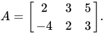
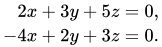
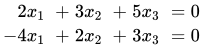
Consider the matrix $${\displaystyle A={\begin{bmatrix}2&3&5\\-4&2&3\end{bmatrix}}.}$$ The kernel of this matrix consists of all vectors (x, y, z) ∈ R³ for which $${\displaystyle {\begin{bmatrix}2&3&5\\-4&2&3\end{bmatrix}}{\begin{bmatrix}x\\y\\z\end{bmatrix}}={\begin{bmatrix}0\\0\end{bmatrix}},}$$ which can be expressed as a homogeneous system of linear equations involving x, y, and z: $${\displaystyle {\begin{aligned}2x+3y+5z&=0,\\-4x+2y+3z&=0.\end{aligned}}}$$

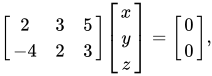
The same linear equations can also be written in matrix form as: $${\displaystyle \left[{\begin{array}{ccc|c}2&3&5&0\\-4&2&3&0\end{array}}\right].}$$

Through Gauss–Jordan elimination, the matrix can be reduced to: $${\displaystyle \left[{\begin{array}{ccc|c}1&0&1/16&0\\0&1&13/8&0\end{array}}\right].}$$

Rewriting the matrix in equation form yields: $${\displaystyle {\begin{aligned}x&=-{\frac {1}{16}}z\\y&=-{\frac {13}{8}}z.\end{aligned}}}$$

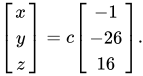
The elements of the kernel can be further expressed in parametric vector form, as follows: $${\displaystyle {\begin{bmatrix}x\\y\\z\end{bmatrix}}=c{\begin{bmatrix}-1/16\\-13/8\\1\end{bmatrix}}\quad ({\text{where }}c\in \mathbb {R} )}$$

Since c is a free variable ranging over all real numbers, this can be expressed equally well as: $${\displaystyle {\begin{bmatrix}x\\y\\z\end{bmatrix}}=c{\begin{bmatrix}-1\\-26\\16\end{bmatrix}}.}$$ The kernel of A is precisely the solution set to these equations (in this case, a line through the origin in R³). Here, the vector (−1,−26,16)^T constitutes a basis of the kernel of A. The nullity of A is therefore 1, as it is spanned by a single vector.

The following dot products are zero: $${\displaystyle {\begin{bmatrix}2&3&5\end{bmatrix}}{\begin{bmatrix}-1\\-26\\16\end{bmatrix}}=0\quad \mathrm {and} \quad {\begin{bmatrix}-4&2&3\end{bmatrix}}{\begin{bmatrix}-1\\-26\\16\end{bmatrix}}=0,}$$ which illustrates that vectors in the kernel of A are orthogonal to each of the row vectors of A.

These two (linearly independent) row vectors span the row space of A—a plane orthogonal to the vector (−1,−26,16)^T.

With the rank 2 of A, the nullity 1 of A, and the dimension 3 of A, we have an illustration of the rank-nullity theorem.

• If L: R^m → Rⁿ, then the kernel of L is the solution set to a homogeneous system of linear equations. As in the above illustration, if L is the operator: $${\displaystyle L(x_{1},x_{2},x_{3})=(2x_{1}+3x_{2}+5x_{3},\;-4x_{1}+2x_{2}+3x_{3})}$$ then the kernel of L is the set of solutions to the equations $${\displaystyle {\begin{alignedat}{7}2x_{1}&\;+\;&3x_{2}&\;+\;&5x_{3}&\;=\;&0\\-4x_{1}&\;+\;&2x_{2}&\;+\;&3x_{3}&\;=\;&0\end{alignedat}}}$$
• Let C[0,1] denote the vector space of all continuous real-valued functions on the interval [0,1], and define L: C[0,1] → R by the rule $${\displaystyle L(f)=f(0.3).}$$ Then the kernel of L consists of all functions f ∈ C[0,1] for which f(0.3) = 0.
• Let C^∞(R) be the vector space of all infinitely differentiable functions R → R, and let D: C^∞(R) → C^∞(R) be the differentiation operator: $${\displaystyle D(f)={\frac {df}{dx}}.}$$ Then the kernel of D consists of all functions in C^∞(R) whose derivatives are zero, i.e. the set of all constant functions.
• Let R^∞ be the direct product of infinitely many copies of R, and let s: R^∞ → R^∞ be the shift operator $${\displaystyle s(x_{1},x_{2},x_{3},x_{4},\ldots )=(x_{2},x_{3},x_{4},\ldots ).}$$ Then the kernel of s is the one-dimensional subspace consisting of all vectors (x₁, 0, 0, 0, ...).
• If V is an inner product space and W is a subspace, the kernel of the orthogonal projection V → W is the orthogonal complement to W in V.

A basis of the kernel of a matrix may be computed by Gaussian elimination.

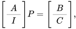
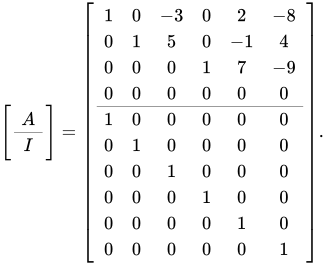
For this purpose, given an m × n matrix A, we construct first the row augmented matrix ${\displaystyle {\begin{bmatrix}A\\\hline I\end{bmatrix}},}$ where I is the n × n identity matrix.

Computing its column echelon form by Gaussian elimination (or any other suitable method), we get a matrix ${\displaystyle {\begin{bmatrix}B\\\hline C\end{bmatrix}}.}$ A basis of the kernel of A consists in the non-zero columns of C such that the corresponding column of B is a zero column.

In fact, the computation may be stopped as soon as the upper matrix is in column echelon form: the remainder of the computation consists in changing the basis of the vector space generated by the columns whose upper part is zero.

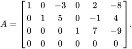
For example, suppose that $${\displaystyle A={\begin{bmatrix}1&0&-3&0&2&-8\\0&1&5&0&-1&4\\0&0&0&1&7&-9\\0&0&0&0&0&0\end{bmatrix}}.}$$ Then $${\displaystyle {\begin{bmatrix}A\\\hline I\end{bmatrix}}={\begin{bmatrix}1&0&-3&0&2&-8\\0&1&5&0&-1&4\\0&0&0&1&7&-9\\0&0&0&0&0&0\\\hline 1&0&0&0&0&0\\0&1&0&0&0&0\\0&0&1&0&0&0\\0&0&0&1&0&0\\0&0&0&0&1&0\\0&0&0&0&0&1\end{bmatrix}}.}$$

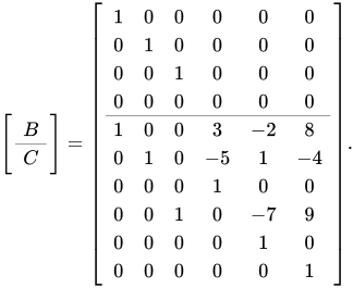
Putting the upper part in column echelon form by column operations on the whole matrix gives $${\displaystyle {\begin{bmatrix}B\\\hline C\end{bmatrix}}={\begin{bmatrix}1&0&0&0&0&0\\0&1&0&0&0&0\\0&0&1&0&0&0\\0&0&0&0&0&0\\\hline 1&0&0&3&-2&8\\0&1&0&-5&1&-4\\0&0&0&1&0&0\\0&0&1&0&-7&9\\0&0&0&0&1&0\\0&0&0&0&0&1\end{bmatrix}}.}$$

The last three columns of B are zero columns. Therefore, the three last vectors of C, $${\displaystyle \left[\!\!{\begin{array}{r}3\\-5\\1\\0\\0\\0\end{array}}\right],\;\left[\!\!{\begin{array}{r}-2\\1\\0\\-7\\1\\0\end{array}}\right],\;\left[\!\!{\begin{array}{r}8\\-4\\0\\9\\0\\1\end{array}}\right]}$$ are a basis of the kernel of A.

Proof that the method computes the kernel: Since column operations correspond to post-multiplication by invertible matrices, the fact that ${\displaystyle {\begin{bmatrix}A\\\hline I\end{bmatrix}}}$ reduces to ${\displaystyle {\begin{bmatrix}B\\\hline C\end{bmatrix}}}$ means that there exists an invertible matrix ${\displaystyle P}$ such that ${\displaystyle {\begin{bmatrix}A\\\hline I\end{bmatrix}}P={\begin{bmatrix}B\\\hline C\end{bmatrix}},}$ with ${\displaystyle B}$ in column echelon form. Thus ${\displaystyle AP=B}$, ${\displaystyle IP=C}$, and ${\displaystyle AC=B}$. A column vector ${\displaystyle \mathbf {v} }$ belongs to the kernel of ${\displaystyle A}$ (that is ${\displaystyle A\mathbf {v} =\mathbf {0} }$) if and only if ${\displaystyle B\mathbf {w} =\mathbf {0} ,}$ where ${\displaystyle \mathbf {w} =P^{-1}\mathbf {v} =C^{-1}\mathbf {v} }$. As ${\displaystyle B}$ is in column echelon form, ${\displaystyle B\mathbf {w} =\mathbf {0} }$, if and only if the nonzero entries of ${\displaystyle \mathbf {w} }$ correspond to the zero columns of ${\displaystyle B}$. By multiplying by ${\displaystyle C}$, one may deduce that this is the case if and only if ${\displaystyle \mathbf {v} =C\mathbf {w} }$ is a linear combination of the corresponding columns of ${\displaystyle C}$.

The problem of computing the kernel on a computer depends on the nature of the coefficients.

If the coefficients of the matrix are exactly given numbers, the column echelon form of the matrix may be computed with Bareiss algorithm more efficiently than with Gaussian elimination. It is even more efficient to use modular arithmetic and Chinese remainder theorem, which reduces the problem to several similar ones over finite fields (this avoids the overhead induced by the non-linearity of the computational complexity of integer multiplication).^{[citation needed]}

For coefficients in a finite field, Gaussian elimination works well, but for the large matrices that occur in cryptography and Gröbner basis computation, better algorithms are known, which have roughly the same computational complexity, but are faster and behave better with modern computer hardware.^{[citation needed]}

For matrices whose entries are floating-point numbers, the problem of computing the kernel makes sense only for matrices such that the number of rows is equal to their rank: because of the rounding errors, a floating-point matrix has almost always a full rank, even when it is an approximation of a matrix of a much smaller rank. Even for a full-rank matrix, it is possible to compute its kernel only if it is well conditioned, i.e. it has a low condition number.^{[5][citation needed]}

Even for a well conditioned full rank matrix, Gaussian elimination does not behave correctly: it introduces rounding errors that are too large for getting a significant result. As the computation of the kernel of a matrix is a special instance of solving a homogeneous system of linear equations, the kernel may be computed with any of the various algorithms designed to solve homogeneous systems. A state of the art software for this purpose is the Lapack library.^{[citation needed]}

Wikibooks has a book on the topic of: Linear Algebra/Null Spaces

• "Kernel of a matrix", Encyclopedia of Mathematics, EMS Press, 2001 [1994]
• Khan Academy, Introduction to the Null Space of a Matrix