Explore Black History

In statistics, kernel density estimation (KDE) is the application of kernel smoothing for probability density estimation, i.e., a non-parametric method to estimate the probability density function of a random variable based on kernels as weights. KDE answers a fundamental data smoothing problem where inferences about the population are made based on a finite data sample. In some fields such as signal processing and econometrics it is also termed the Parzen–Rosenblatt window method, after Emanuel Parzen and Murray Rosenblatt, who are usually credited with independently creating it in its current form.^[1][2] One of the famous applications of kernel density estimation is in estimating the class-conditional marginal densities of data when using a naive Bayes classifier, which can improve its prediction accuracy.^[3]

Let ${\displaystyle \mathbf {x} =\left(x_{1},x_{2},x_{3},...\right)}$ be independent and identically distributed samples drawn from some univariate distribution with an unknown density f at any given point x. We are interested in estimating the shape of this function f. Its kernel density estimator is $${\displaystyle {\hat {f}}_{h}(x)={\frac {1}{n}}\sum _{i=1}^{n}K_{h}(x-x_{i})={\frac {1}{nh}}\sum _{i=1}^{n}K{\left({\frac {x-x_{i}}{h}}\right)},}$$ where K is the kernel — a non-negative function — and h > 0 is a smoothing parameter called the bandwidth or simply width.^[3] A kernel with subscript h is called the scaled kernel and defined as K_h(x) = ⁠1/h⁠ K(⁠x/h⁠). Intuitively one wants to choose h as small as the data will allow; however, there is always a trade-off between the bias of the estimator and its variance. The choice of bandwidth is discussed in more detail below.

A range of kernel functions are commonly used: uniform, triangular, biweight, triweight, Epanechnikov (parabolic), normal, and others. The Epanechnikov kernel is optimal in a mean square error sense,^[4] though the loss of efficiency is small for the kernels listed previously.^[5] Due to its convenient mathematical properties, the normal kernel is often used, which means K(x) = ϕ(x), where ϕ is the standard normal density function. The kernel density estimator then becomes $${\displaystyle {\hat {f}}_{h}(x)={\frac {1}{n}}\sum _{i=1}^{n}{\frac {1}{h{\sqrt {2\pi }}}}\exp \left({\frac {-(x-x_{i})^{2}}{2h^{2}}}\right),}$$ where ${\displaystyle h}$ is the standard deviation of the sample ${\displaystyle \mathbf {x} }$.

The construction of a kernel density estimate finds interpretations in fields outside of density estimation.^[6] For example, in thermodynamics, this is equivalent to the amount of heat generated when heat kernels (the fundamental solution to the heat equation) are placed at each data point locations x_i. Similar methods are used to construct discrete Laplace operators on point clouds for manifold learning (e.g. diffusion map).

Kernel density estimates are closely related to histograms, but can be endowed with properties such as smoothness or continuity by using a suitable kernel. The diagram below based on these 6 data points illustrates this relationship:

For the histogram, first, the horizontal axis is divided into sub-intervals or bins which cover the range of the data: In this case, six bins each of width 2. Whenever a data point falls inside this interval, a box of height 1/12 is placed there. If more than one data point falls inside the same bin, the boxes are stacked on top of each other.

For the kernel density estimate, normal kernels with a standard deviation of 1.5 (indicated by the red dashed lines) are placed on each of the data points x_i. The kernels are summed to make the kernel density estimate (solid blue curve). The smoothness of the kernel density estimate (compared to the discreteness of the histogram) illustrates how kernel density estimates converge faster to the true underlying density for continuous random variables.^[7]

The bandwidth of the kernel is a free parameter which exhibits a strong influence on the resulting estimate. To illustrate its effect, we take a simulated random sample from the standard normal distribution (plotted at the blue spikes in the rug plot on the horizontal axis). The grey curve is the true density (a normal density with mean 0 and variance 1). In comparison, the red curve is undersmoothed since it contains too many spurious data artifacts arising from using a bandwidth h = 0.05, which is too small. The green curve is oversmoothed since using the bandwidth h = 2 obscures much of the underlying structure. The black curve with a bandwidth of h = 0.337 is considered to be optimally smoothed since its density estimate is close to the true density. An extreme situation is encountered in the limit ${\displaystyle h\to 0}$ (no smoothing), where the estimate is a sum of n delta functions centered at the coordinates of analyzed samples. In the other extreme limit ${\displaystyle h\to \infty }$ the estimate retains the shape of the used kernel, centered on the mean of the samples (completely smooth).

The most common optimality criterion used to select this parameter is the expected L₂ risk function, also termed the mean integrated squared error:

$${\displaystyle \operatorname {MISE} (h)=\operatorname {E} \!\left[\int \!{\left({\hat {f}}\!_{h}(x)-f(x)\right)}^{2}dx\right]}$$

Under weak assumptions on f and K, (f is the, generally unknown, real density function),^[1][2]

$${\displaystyle \operatorname {MISE} (h)=\operatorname {AMISE} (h)+{\mathcal {o}}{\left((nh)^{-1}+h^{4}\right)}}$$

where o is the little o notation, and n the sample size (as above). The AMISE is the asymptotic MISE, i. e. the two leading terms,

$${\displaystyle \operatorname {AMISE} (h)={\frac {R(K)}{nh}}+{\frac {1}{4}}m_{2}(K)^{2}h^{4}R(f'')}$$

where ${\textstyle R(g)=\int g(x)^{2}\,dx}$ for a function g, ${\textstyle m_{2}(K)=\int x^{2}K(x)\,dx}$ and ${\displaystyle f''}$ is the second derivative of ${\displaystyle f}$ and ${\displaystyle K}$ is the kernel. The minimum of this AMISE is the solution to this differential equation

$${\displaystyle {\frac {\partial }{\partial h}}\operatorname {AMISE} (h)=-{\frac {R(K)}{nh^{2}}}+m_{2}(K)^{2}h^{3}R(f'')=0}$$

or

$${\displaystyle h_{\operatorname {AMISE} }={\frac {R(K)^{1/5}}{m_{2}(K)^{2/5}R(f'')^{1/5}}}n^{-1/5}=Cn^{-1/5}}$$

Neither the AMISE nor the h_AMISE formulas can be used directly since they involve the unknown density function ${\displaystyle f}$ or its second derivative ${\displaystyle f''}$. To overcome that difficulty, a variety of automatic, data-based methods have been developed to select the bandwidth. Several review studies have been undertaken to compare their efficacies,^{[8][9][10][11][12][13][14]} with the general consensus that the plug-in selectors^[6][15][16] and cross validation selectors^[17][18][19] are the most useful over a wide range of data sets.

Substituting any bandwidth h which has the same asymptotic order n^−1/5 as h_AMISE into the AMISE gives that AMISE(h) = O(n^−4/5), where O is the big O notation. It can be shown that, under weak assumptions, there cannot exist a non-parametric estimator that converges at a faster rate than the kernel estimator.^[20] Note that the n^−4/5 rate is slower than the typical n⁻¹ convergence rate of parametric methods.

If the bandwidth is not held fixed, but is varied depending upon the location of either the estimate (balloon estimator) or the samples (pointwise estimator), this produces a particularly powerful method termed adaptive or variable bandwidth kernel density estimation.

Bandwidth selection for kernel density estimation of heavy-tailed distributions is relatively difficult.^[21]

If Gaussian basis functions are used to approximate univariate data, and the underlying density being estimated is Gaussian, the optimal choice for h (that is, the bandwidth that minimises the mean integrated squared error) is:^[22]

$${\displaystyle h={\left({\frac {4{\hat {\sigma }}^{5}}{3n}}\right)}^{1/5}\approx 1.06\,{\hat {\sigma }}\,n^{-1/5},}$$

An ${\displaystyle h}$ value is considered more robust when it improves the fit for long-tailed and skewed distributions or for bimodal mixture distributions. This is often done empirically by replacing the standard deviation ${\displaystyle {\hat {\sigma }}}$ by the parameter ${\displaystyle A}$ below:

$${\displaystyle A=\min \left({\hat {\sigma }},{\frac {\mathrm {IQR} }{1.34}}\right)}$$ where IQR is the interquartile range.

Another modification that will improve the model is to reduce the factor from 1.06 to 0.9. Then the final formula would be:

$${\displaystyle h=0.9\,\min \left({\hat {\sigma }},{\frac {\mathrm {IQR} }{1.34}}\right)\,n^{-1/5}}$$ where ${\displaystyle n}$ is the sample size.

This approximation is termed the normal distribution approximation, Gaussian approximation, or Silverman's rule of thumb.^[22] While this rule of thumb is easy to compute, it should be used with caution as it can yield widely inaccurate estimates when the density is not close to being normal. For example, when estimating the bimodal Gaussian mixture model $${\displaystyle {\frac {1}{2{\sqrt {2\pi }}}}e^{-{\frac {1}{2}}(x-10)^{2}}+{\frac {1}{2{\sqrt {2\pi }}}}e^{-{\frac {1}{2}}(x+10)^{2}}}$$ from a sample of 200 points, the figure on the right shows the true density and two kernel density estimates — one using the rule-of-thumb bandwidth, and the other using a solve-the-equation bandwidth.^[6][16] The estimate based on the rule-of-thumb bandwidth is significantly oversmoothed.

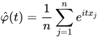
Given the sample (x₁, x₂, ..., x_n), it is natural to estimate the characteristic function φ(t) = E[e^itX] as $${\displaystyle {\hat {\varphi }}(t)={\frac {1}{n}}\sum _{j=1}^{n}e^{itx_{j}}}$$ Knowing the characteristic function, it is possible to find the corresponding probability density function through the Fourier transform formula. One difficulty with applying this inversion formula is that it leads to a diverging integral, since the estimate ${\displaystyle {\hat {\varphi }}(t)}$ is unreliable for large t's. To circumvent this problem, the estimator ${\displaystyle {\hat {\varphi }}(t)}$ is multiplied by a damping function ψ_h(t) = ψ(ht), which is equal to 1 at the origin and then falls to 0 at infinity. The "bandwidth parameter" h controls how fast we try to dampen the function ${\displaystyle {\hat {\varphi }}(t)}$. In particular when h is small, then ψ_h(t) will be approximately one for a large range of t's, which means that ${\displaystyle {\hat {\varphi }}(t)}$ remains practically unaltered in the most important region of t's.

The most common choice for function ψ is either the uniform function ψ(t) = 1{−1 ≤ t ≤ 1}, which effectively means truncating the interval of integration in the inversion formula to [−1/h, 1/h], or the Gaussian function ψ(t) = e^−πt2. Once the function ψ has been chosen, the inversion formula may be applied, and the density estimator will be $${\displaystyle {\begin{aligned}{\hat {f}}(x)&={\frac {1}{2\pi }}\int _{-\infty }^{+\infty }{\hat {\varphi }}(t)\psi _{h}(t)e^{-itx}\,dt\\[1ex]&={\frac {1}{2\pi }}\int _{-\infty }^{+\infty }{\frac {1}{n}}\sum _{j=1}^{n}e^{it(x_{j}-x)}\psi (ht)\,dt\\[1ex]&={\frac {1}{nh}}\sum _{j=1}^{n}{\frac {1}{2\pi }}\int _{-\infty }^{+\infty }e^{-i(ht){\frac {x-x_{j}}{h}}}\psi (ht)\,d(ht)\\[1ex]&={\frac {1}{nh}}\sum _{j=1}^{n}K{\left({\frac {x-x_{j}}{h}}\right)},\end{aligned}}}$$

where K is the Fourier transform of the damping function ψ. Thus the kernel density estimator coincides with the characteristic function density estimator.

Kernel density estimation has been applied to continuous-variable quantum state tomography, in which repeated homodyne measurements produce samples of rotated field quadratures. For real measurement parameters ${\displaystyle (\mu ,\nu )}$, the quadrature observable is

${\displaystyle X_{\mu ,\nu }=\mu q+\nu p.}$

Its measurement outcomes follow an ordinary probability density ${\displaystyle {\mathcal {W}}(x\mid \mu ,\nu )}$, known as a symplectic tomogram. The collection of tomograms over different measurement settings is informationally complete and therefore provides an alternative representation of the quantum state.^[23]

For independent quadrature measurements ${\displaystyle X_{1,\mu ,\nu },\ldots ,X_{n,\mu ,\nu }}$ obtained at a fixed setting, the tomogram can be estimated by

${\displaystyle {\widehat {\mathcal {W}}}_{n,h}(x\mid \mu ,\nu )={\frac {1}{nh}}\sum _{j=1}^{n}K_{\mu ,\nu }\left({\frac {x-X_{j,\mu ,\nu }}{h}}\right),}$

where ${\displaystyle K_{\mu ,\nu }}$ is a kernel and ${\displaystyle h}$ is the bandwidth. This treatment does not require the quadrature density to belong to a predetermined parametric family and can therefore accommodate multimodal and non-Gaussian measurement distributions.

The characteristic function of a tomogram is its Fourier transform,

${\displaystyle \varphi (t;\mu ,\nu )=\int _{-\infty }^{\infty }{\mathcal {W}}(x\mid \mu ,\nu )e^{itx}\,dx.}$

For every fixed ${\displaystyle (\mu ,\nu )}$, this is the characteristic function of the measured random variable ${\displaystyle X_{\mu ,\nu }}$. It always exists and satisfies the standard conditions ${\displaystyle \varphi (0;\mu ,\nu )=1}$, ${\displaystyle |\varphi (t;\mu ,\nu )|\leq 1}$, and ${\displaystyle \varphi (-t;\mu ,\nu )=\varphi (t;\mu ,\nu )^{*}}$. In the tomographic representation, the values ${\displaystyle \varphi (1;\mu ,\nu )}$ over phase space also coincide, up to the adopted conventions, with the characteristic function associated with the Wigner representation of the state.^[23]

Taking the Fourier transform of the kernel density estimator gives a kernel estimator of the characteristic function,

${\displaystyle {\widehat {\varphi }}_{n,h}(t;\mu ,\nu )={\widehat {\varphi }}_{X,n}(t;\mu ,\nu )\varphi _{K}(th;\mu ,\nu ),}$

where

${\displaystyle {\widehat {\varphi }}_{X,n}(t;\mu ,\nu )={\frac {1}{n}}\sum _{j=1}^{n}e^{itX_{j,\mu ,\nu }}}$

is the empirical characteristic function and

${\displaystyle \varphi _{K}(th;\mu ,\nu )=\int _{-\infty }^{\infty }K_{\mu ,\nu }(z)e^{ithz}\,dz}$

is the known characteristic function of the rescaled kernel. Thus, the estimator separates into a data-dependent empirical factor and a deterministic smoothing factor controlled by the kernel and bandwidth. The kernel factor suppresses high-frequency contributions, providing a regularized version of the empirical characteristic function.

The characteristic-function representation can be used directly for quantum-state reconstruction. For example, the density matrix in the coordinate basis can be recovered from

${\displaystyle \rho (y,y')={\frac {1}{2\pi }}\int _{-\infty }^{\infty }\varphi (1;\mu ,y-y')\exp \left[-{\frac {i\mu (y+y')}{2}}\right]\,d\mu .}$

It can also be used to calculate trace quantities without first reconstructing a phase-space quasiprobability distribution. In particular, two density operators satisfy the Parseval-type relation

${\displaystyle \operatorname {tr} (\rho _{1}\rho _{2})={\frac {1}{2\pi }}\iint _{\mathbb {R} ^{2}}\varphi _{1}(1;\mu ,\nu )\varphi _{2}(1;\mu ,\nu )^{*}\,d\mu \,d\nu .}$

When the two states are identical, this expression gives the purity ${\displaystyle \operatorname {tr} (\rho ^{2})}$; for different states it gives their Hilbert–Schmidt overlap. Related integral expressions can be constructed for higher-order traces, state distances, and phase-space quasiprobability distributions.^[23]

The characteristic-function formulation also permits correction for some measurement-noise models. If the observed quadrature is modeled as ${\displaystyle Z=\kappa X+(1-\kappa )Y}$, where ${\displaystyle Y}$ is independent noise with a known nonvanishing characteristic function, then the signal characteristic function can be obtained through a deconvolution,

${\displaystyle \varphi _{X}(t)={\frac {\varphi _{Z}(t/\kappa )}{\varphi _{Y}((1-\kappa )t/\kappa )}}.}$

A kernel factor can subsequently be included to regularize the resulting estimate. This correction requires the noise characteristic function not to vanish at the frequencies used in the reconstruction.

The bias and variance of the KCFE are

${\displaystyle \operatorname {Bias} \!\left[{\widehat {\varphi }}_{n,h}(t;\mu ,\nu )\right]=\left[\varphi _{K}(th;\mu ,\nu )-1\right]\varphi (t;\mu ,\nu )}$

and

${\displaystyle \operatorname {Var} \!\left[{\widehat {\varphi }}_{n,h}(t;\mu ,\nu )\right]={\frac {|\varphi _{K}(th;\mu ,\nu )|^{2}}{n}}\left[1-|\varphi (t;\mu ,\nu )|^{2}\right].}$

Thus its pointwise mean squared error is

${\displaystyle {\begin{aligned}\operatorname {MSE} \!\left[{\widehat {\varphi }}_{n,h}(t;\mu ,\nu )\right]={}&|\varphi _{K}(th;\mu ,\nu )-1|^{2}|\varphi (t;\mu ,\nu )|^{2}\\&+{\frac {|\varphi _{K}(th;\mu ,\nu )|^{2}}{n}}\left[1-|\varphi (t;\mu ,\nu )|^{2}\right].\end{aligned}}}$

For the Gaussian kernel

${\displaystyle \varphi _{K}(th;\mu ,\nu )=\exp \left[-{\frac {t^{2}h^{2}(\mu ^{2}+\nu ^{2})}{4}}\right].}$

The resulting error is

${\displaystyle {\begin{aligned}\operatorname {MSE} \!\left[{\widehat {\varphi }}_{n,h}^{\,G}(t;\mu ,\nu )\right]={}&\left(\exp \left[-{\frac {t^{2}h^{2}(\mu ^{2}+\nu ^{2})}{4}}\right]-1\right)^{2}|\varphi (t;\mu ,\nu )|^{2}\\&+{\frac {1}{n}}\exp \left[-{\frac {t^{2}h^{2}(\mu ^{2}+\nu ^{2})}{4}}\right]\left[1-|\varphi (t;\mu ,\nu )|^{2}\right].\end{aligned}}}$

For ${\displaystyle 0<|\varphi (t;\mu ,\nu )|<1}$, minimizing this expression gives a characteristic-function bandwidth of order

${\displaystyle h_{\varphi }=O(n^{-1/2}),}$

and the minimized error satisfies

${\displaystyle \operatorname {MSE} \!\left[{\widehat {\varphi }}_{n,h_{\varphi }}^{\,G}(t;\mu ,\nu )\right]={\frac {1-|\varphi (t;\mu ,\nu )|^{2}}{n}}-{\frac {\left[1-|\varphi (t;\mu ,\nu )|^{2}\right]^{2}}{4n^{2}|\varphi (t;\mu ,\nu )|^{2}}}=O(n^{-1}).}$

The characteristic-function estimator therefore converges pointwise at the parametric ${\displaystyle n^{-1}}$ mean squared error rate, although the underlying tomogram is estimated nonparametrically.^[23]

Collections of characteristic-function estimates at several measurement settings form the input to the kernel quantum state estimation procedure. If ${\displaystyle n}$ measurements are taken at each setting and ${\displaystyle N_{\mu }=N_{\nu }=(\log n)^{2}}$, the numbers of state preparations used for density-matrix and two-dimensional trace estimation are

${\displaystyle T_{\mu }=nN_{\mu },\qquad T_{\mu ,\nu }=nN_{\mu }N_{\nu }.}$

For the coordinate-space density matrix, the reported uniform pointwise risk is

${\displaystyle \sup _{y,y'}\mathbb {E} \left[\left|{\widehat {\rho }}(y,y')-\rho (y,y')\right|^{2}\right]={\widetilde {O}}\!\left(T_{\mu }^{-1}\right).}$

For the overlap of two quantum states, the reported mean squared error is

${\displaystyle \mathbb {E} \left[\left|{\widehat {\operatorname {tr} (\rho _{1}\rho _{2})}}-\operatorname {tr} (\rho _{1}\rho _{2})\right|^{2}\right]={\widetilde {O}}\!\left(T_{\mu ,\nu }^{-1}\right),}$

where ${\displaystyle {\widetilde {O}}}$ suppresses logarithmic factors arising from the number of measurement settings.^[23]

We can extend the definition of the (global) mode to a local sense and define the local modes:

$${\displaystyle M=\{x:g(x)=0\mid \lambda _{1}(x)<0\}}$$

Namely, ${\displaystyle M}$ is the collection of points for which the density function is locally maximized. A natural estimator of ${\displaystyle M}$ is a plug-in from KDE,^[24][25] where ${\displaystyle g(x)}$ and ${\displaystyle \lambda _{1}(x)}$ are KDE version of ${\displaystyle g(x)}$ and ${\displaystyle \lambda _{1}(x)}$. Under mild assumptions, ${\displaystyle M_{c}}$ is a consistent estimator of ${\displaystyle M}$. Note that one can use the mean shift algorithm^[26][27][28] to compute the estimator ${\displaystyle M_{c}}$ numerically.

A non-exhaustive list of software implementations of kernel density estimators includes:

• In Analytica release 4.4, the Smoothing option for PDF results uses KDE, and from expressions it is available via the built-in Pdf function.
• In C/C++, FIGTree is a library that can be used to compute kernel density estimates using normal kernels. MATLAB interface available.
• In C++, libagf is a library for variable kernel density estimation.
• In C++, mlpack is a library that can compute KDE using many different kernels. It allows to set an error tolerance for faster computation. Python and R interfaces are available.
• in C# and F#, Math.NET Numerics is an open source library for numerical computation which includes kernel density estimation
• In CrimeStat, kernel density estimation is implemented using five different kernel functions – normal, uniform, quartic, negative exponential, and triangular. Both single- and dual-kernel density estimate routines are available. Kernel density estimation is also used in interpolating a Head Bang routine, in estimating a two-dimensional Journey-to-crime density function, and in estimating a three-dimensional Bayesian Journey-to-crime estimate.
• In ELKI, kernel density functions can be found in the package de.lmu.ifi.dbs.elki.math.statistics.kernelfunctions
• In ESRI products, kernel density mapping is managed out of the Spatial Analyst toolbox and uses the Quartic(biweight) kernel.
• In Excel, the Royal Society of Chemistry has created an add-in to run kernel density estimation based on their Analytical Methods Committee Technical Brief 4.
• In gnuplot, kernel density estimation is implemented by the smooth kdensity option, the datafile can contain a weight and bandwidth for each point, or the bandwidth can be set automatically^[29] according to "Silverman's rule of thumb" (see above).
• In Haskell, kernel density is implemented in the statistics package.
• In IGOR Pro, kernel density estimation is implemented by the StatsKDE operation (added in Igor Pro 7.00). Bandwidth can be user specified or estimated by means of Silverman, Scott or Bowmann and Azzalini. Kernel types are: Epanechnikov, Bi-weight, Tri-weight, Triangular, Gaussian and Rectangular.
• In Java, the Weka machine learning package provides weka.estimators.KernelEstimator, among others.
• In JavaScript, the visualization package D3.js offers a KDE package in its science.stats package.
• In JMP, the Graph Builder platform utilizes kernel density estimation to provide contour plots and high density regions (HDRs) for bivariate densities, and violin plots and HDRs for univariate densities. Sliders allow the user to vary the bandwidth. Bivariate and univariate kernel density estimates are also provided by the Fit Y by X and Distribution platforms, respectively.
• In Julia, kernel density estimation is implemented in the KernelDensity.jl package.
• In KNIME, 1D and 2D Kernel Density distributions can be generated and plotted using nodes from the Vernalis community contribution, e.g. 1D Kernel Density Plot, among others. The underlying implementation is written in Java.
• In MATLAB, kernel density estimation is implemented through the ksdensity function (Statistics Toolbox). As of the 2018a release of MATLAB, both the bandwidth and kernel smoother can be specified, including other options such as specifying the range of the kernel density.^[30] Alternatively, a free MATLAB software package which implements an automatic bandwidth selection method^[6] is available from the MATLAB Central File Exchange for
  • 1-dimensional data
  • 2-dimensional data
  • n-dimensional data Archived 2017-02-09 at the Wayback Machine
    A free MATLAB toolbox with implementation of kernel regression, kernel density estimation, kernel estimation of hazard function and many others is available on these pages (this toolbox is a part of the book ^[31]).
• In Mathematica, numeric kernel density estimation is implemented by the function SmoothKernelDistribution^[32] and symbolic estimation is implemented using the function KernelMixtureDistribution^[33] both of which provide data-driven bandwidths.
• In Minitab, the Royal Society of Chemistry has created a macro to run kernel density estimation based on their Analytical Methods Committee Technical Brief 4.^[34]
• In the NAG Library, kernel density estimation is implemented via the g10ba routine (available in both the Fortran^[35] and the C^[36] versions of the Library).
• In Nuklei, C++ kernel density methods focus on data from the Special Euclidean group ${\displaystyle SE(3)}$.
• In Octave, kernel density estimation is implemented by the kernel_density option (econometrics package).
• In Origin, 2D kernel density plot can be made from its user interface, and two functions, Ksdensity for 1D and Ks2density for 2D can be used from its LabTalk Archived 2014-10-19 at the Wayback Machine, Python, or C code.
• In Perl, an implementation can be found in the Statistics-KernelEstimation module
• In PHP, an implementation can be found in the MathPHP library
• In Python, many implementations exist: pyqt_fit.kde Module in the PyQt-Fit package, SciPy (scipy.stats.gaussian_kde), Statsmodels (KDEUnivariate and KDEMultivariate), and scikit-learn (KernelDensity) (see comparison^[37]). KDEpy supports weighted data and its FFT implementation is orders of magnitude faster than the other implementations. The commonly used pandas library [1] offers support for kde plotting through the plot method (df.plot(kind='kde')[2]). The getdist package for weighted and correlated MCMC samples supports optimized bandwidth, boundary correction and higher-order methods for 1D and 2D distributions. One newly used package for kernel density estimation is seaborn ( import seaborn as sns , sns.kdeplot() ).^[38] A GPU implementation of KDE also exists.^[39]
• In R, it is implemented through density in the base distribution, and bw.nrd0 function is used in stats package, this function uses the optimized formula in Silverman's book. bkde in the KernSmooth library, ParetoDensityEstimation in the DataVisualizations library (for pareto distribution density estimation), kde in the ks library, dkden and dbckden in the evmix library (latter for boundary corrected kernel density estimation for bounded support), npudens in the np library (numeric and categorical data), sm.density in the sm library. For an implementation of the kde.R function, which does not require installing any packages or libraries, see kde.R. The btb library, dedicated to urban analysis, implements kernel density estimation through kernel_smoothing.
• In SAS, proc kde can be used to estimate univariate and bivariate kernel densities.
• In Apache Spark, the KernelDensity() class^[40]
• In Stata, it is implemented through kdensity;^[41] for example histogram x, kdensity. Alternatively a free Stata module KDENS is available^[42] allowing a user to estimate 1D or 2D density functions.
• In Swift, it is implemented through SwiftStats.KernelDensityEstimation in the open-source statistics library SwiftStats.

Wikimedia Commons has media related to Kernel density estimation.

• Kernel (statistics)
• Kernel smoothing
• Kernel regression
• Density estimation (with presentation of other examples)
• Mean-shift
• Scale space: The triplets {(x, h, KDE with bandwidth h evaluated at x: all x, h > 0} form a scale space representation of the data.
• Multivariate kernel density estimation
• Variable kernel density estimation
• Head/tail breaks

• Härdle, Wolfgang; Müller, Marlene; Sperlich, Stefan; Werwatz, Axel (2004). Nonparametric and Semiparametric Models. Springer Series in Statistics. Berlin Heidelberg: Springer-Verlag. pp. 39–83. ISBN 978-3-540-20722-1.

• Introduction to kernel density estimation A short tutorial which motivates kernel density estimators as an improvement over histograms.
• Kernel Bandwidth Optimization A free online tool that generates an optimized kernel density estimate.
• Free Online Software (Calculator) computes the Kernel Density Estimation for a data series according to the following Kernels: Gaussian, Epanechnikov, Rectangular, Triangular, Biweight, Cosine, and Optcosine.
• Kernel Density Estimation Applet An online interactive example of kernel density estimation. Requires .NET 3.0 or later.