Explore Black History

This article needs more citations. Please help improve this article by adding citations to reliable sources. Unsourced material may be challenged and removed. Find sources: "Line integral" – news · newspapers · books · scholar · JSTOR (June 2023) (Learn how and when to remove this message)

In mathematics, a line integral is an integral where the function to be integrated is evaluated along a curve.^[1] The terms path integral, curve integral, and curvilinear integral are also used; contour integral is used as well, although that is typically reserved for line integrals in the complex plane.

The function to be integrated may be a scalar field or a vector field. The value of the line integral is the sum of values of the field at all points on the curve, weighted by some scalar function on the curve (commonly arc length or, for a vector field, the scalar product of the vector field with a differential vector in the curve). This weighting distinguishes the line integral from simpler integrals defined on intervals. Many simple formulae in physics, such as the definition of work as ${\displaystyle W=\mathbf {F} \cdot \mathbf {s} }$, have natural continuous analogues in terms of line integrals, in this case ${\textstyle W=\int _{L}\mathbf {F} (\mathbf {s} )\cdot d\mathbf {s} }$, which computes the work done on an object moving through an electric or gravitational field F along a path ${\displaystyle L}$.

In qualitative terms, a line integral in vector calculus can be thought of as a measure of the total effect of a given tensor field along a given curve. For example, the line integral over a scalar field (rank 0 tensor) can be interpreted as the area under the field carved out by a particular curve. This can be visualized as the surface created by z = f(x,y) and a curve C in the xy plane. The line integral of f would be the area of the "curtain" created—when the points of the surface that are directly over C are carved out.

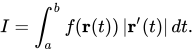
For some scalar field ${\displaystyle f\colon U\to \mathbb {R} }$ where ${\displaystyle U\subseteq \mathbb {R} ^{n}}$, the line integral along a piecewise smooth curve ${\displaystyle {\mathcal {C}}\subset U}$ is defined as $${\displaystyle \int _{\mathcal {C}}f\,ds=\int _{a}^{b}f\left(\mathbf {r} (t)\right)\left|\mathbf {r} '(t)\right|\,dt,}$$ where ${\displaystyle \mathbf {r} \colon [a,b]\to {\mathcal {C}}}$ is an arbitrary bijective parametrization of the curve ${\displaystyle {\mathcal {C}}}$ such that r(a) and r(b) give the endpoints of ${\displaystyle {\mathcal {C}}}$ and a < b. Here, and in the rest of the article, the absolute value bars denote the standard (Euclidean) norm of a vector.

The function f is called the integrand, the curve ${\displaystyle {\mathcal {C}}}$ is the domain of integration, and the symbol ds may be intuitively interpreted as an elementary arc length of the curve ${\displaystyle {\mathcal {C}}}$ (i.e., a differential length of ${\displaystyle {\mathcal {C}}}$). Line integrals of scalar fields over a curve ${\displaystyle {\mathcal {C}}}$ do not depend on the chosen parametrization r of ${\displaystyle {\mathcal {C}}}$.^[2]

Geometrically, when the scalar field f is defined over a plane (n = 2), its graph is a surface z = f(x, y) in space, and the line integral gives the (signed) cross-sectional area bounded by the curve ${\displaystyle {\mathcal {C}}}$ and the graph of f. See the animation to the right.

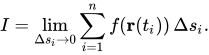
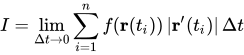
For a line integral over a scalar field, the integral can be constructed from a Riemann sum using the above definitions of f, C and a parametrization r of C. This can be done by partitioning the interval [a, b] into n sub-intervals [t_i−1, t_i] of length Δt = (b − a)/n, then r(t_i) denotes some point, call it a sample point, on the curve C. We can use the set of sample points {r(t_i): 1 ≤ i ≤ n} to approximate the curve C as a polygonal path by introducing the straight line piece between each of the sample points r(t_i−1) and r(t_i). (The approximation of a curve to a polygonal path is called rectification of a curve, see here for more details.) We then label the distance of the line segment between adjacent sample points on the curve as Δs_i. The product of f(r(t_i)) and Δs_i can be associated with the signed area of a rectangle with a height and width of f(r(t_i)) and Δs_i, respectively. Taking the limit of the sum of the terms as the length of the partitions approaches zero gives us $${\displaystyle I=\lim _{\Delta s_{i}\to 0}\sum _{i=1}^{n}f(\mathbf {r} (t_{i}))\,\Delta s_{i}.}$$

By the mean value theorem, the distance between subsequent points on the curve, is $${\displaystyle \Delta s_{i}=\left|\mathbf {r} (t_{i}+\Delta t)-\mathbf {r} (t_{i})\right|\approx \left|\mathbf {r} '(t_{i})\Delta t\right|}$$

Substituting this in the above Riemann sum yields $${\displaystyle I=\lim _{\Delta t\to 0}\sum _{i=1}^{n}f(\mathbf {r} (t_{i}))\left|\mathbf {r} '(t_{i})\right|\Delta t}$$ which is the Riemann sum for the integral $${\displaystyle I=\int _{a}^{b}f(\mathbf {r} (t))\left|\mathbf {r} '(t)\right|dt.}$$

For a vector field F: U ⊆ Rⁿ → Rⁿ, the line integral along a piecewise smooth curve C ⊂ U, in the direction of r, is defined as $${\displaystyle \int _{C}\mathbf {F} (\mathbf {r} )\cdot d\mathbf {r} =\int _{a}^{b}\mathbf {F} (\mathbf {r} (t))\cdot \mathbf {r} '(t)\,dt}$$ where · is the dot product, and r: [a, b] → C is a regular parametrization (i.e: ${\displaystyle ||\mathbf {r} '(t)||\neq 0\;\;\forall t\in [a,b]}$) of the curve C such that r(a) and r(b) give the endpoints of C.

A line integral of a scalar field is thus a line integral of a vector field, where the vectors are always tangential to the line of the integration.

Line integrals of vector fields are independent of the parametrization r in absolute value, but they do depend on its orientation. Specifically, a reversal in the orientation of the parametrization changes the sign of the line integral.^[2]

From the viewpoint of differential geometry, the line integral of a vector field along a curve is the integral of the corresponding 1-form under the musical isomorphism (which takes the vector field to the corresponding covector field), over the curve considered as an immersed 1-manifold.

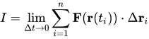
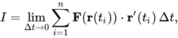
The line integral of a vector field can be derived in a manner very similar to the case of a scalar field, but this time with the inclusion of a dot product. Again using the above definitions of F, C and its parametrization r(t), we construct the integral from a Riemann sum. We partition the interval [a, b] (which is the range of the values of the parameter t) into n intervals of length Δt = (b − a)/n. Letting t_i be the ith point on [a, b], then r(t_i) gives us the position of the ith point on the curve. However, instead of calculating up the distances between subsequent points, we need to calculate their displacement vectors, Δr_i. As before, evaluating F at all the points on the curve and taking the dot product with each displacement vector gives us the infinitesimal contribution of each partition of F on C. Letting the size of the partitions go to zero gives us a sum $${\displaystyle I=\lim _{\Delta t\to 0}\sum _{i=1}^{n}\mathbf {F} (\mathbf {r} (t_{i}))\cdot \Delta \mathbf {r} _{i}}$$

By the mean value theorem, we see that the displacement vector between adjacent points on the curve is $${\displaystyle \Delta \mathbf {r} _{i}=\mathbf {r} (t_{i}+\Delta t)-\mathbf {r} (t_{i})\approx \mathbf {r} '(t_{i})\,\Delta t.}$$

Substituting this in the above Riemann sum yields $${\displaystyle I=\lim _{\Delta t\to 0}\sum _{i=1}^{n}\mathbf {F} (\mathbf {r} (t_{i}))\cdot \mathbf {r} '(t_{i})\,\Delta t,}$$

which is the Riemann sum for the integral defined above.

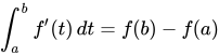
If a vector field F is the gradient of a scalar field G (i.e. if F is conservative), that is, $${\displaystyle \mathbf {F} =\nabla G,}$$ then by the multivariable chain rule the derivative of the composition of G and r(t) is $${\displaystyle {\frac {dG(\mathbf {r} (t))}{dt}}=\nabla G(\mathbf {r} )\cdot \mathbf {r} '(t)=\mathbf {F} (\mathbf {r} (t))\cdot \mathbf {r} '(t)}$$ which happens to be the integrand for the line integral of F on r(t). It follows, given a path C, that $${\displaystyle \int _{C}\mathbf {F} (\mathbf {r} )\cdot d\mathbf {r} =\int _{a}^{b}\mathbf {F} (\mathbf {r} (t))\cdot \mathbf {r} '(t)\,dt=\int _{a}^{b}{\frac {dG(\mathbf {r} (t))}{dt}}\,dt=G(\mathbf {r} (b))-G(\mathbf {r} (a)).}$$

In other words, the integral of F over C depends solely on the values of G at the points r(b) and r(a), and is thus independent of the path between them. For this reason, a line integral of a conservative vector field is called path independent.

The line integral has many uses in physics. For example, the work done on a particle traveling on a curve C inside a force field represented as a vector field F is the line integral of F on C.^[3]

For another example, see Ampère's circuital law.

For a vector field ${\displaystyle \mathbf {F} \colon U\subseteq \mathbb {R} ^{2}\to \mathbb {R} ^{2}}$, F(x, y) = (P(x, y), Q(x, y)), the line integral across a curve C ⊂ U, also called the flux integral, is defined in terms of a piecewise smooth parametrization r: [a,b] → C, r(t) = (x(t), y(t)), as: $${\displaystyle \int _{C}\mathbf {F} (\mathbf {r} )\cdot d\mathbf {r} ^{\perp }=\int _{a}^{b}{\begin{bmatrix}P{\big (}x(t),y(t){\big )}\\Q{\big (}x(t),y(t){\big )}\end{bmatrix}}\cdot {\begin{bmatrix}y'(t)\\-x'(t)\end{bmatrix}}~dt=\int _{a}^{b}\left(-Q~dx+P~dy\right).}$$

Here ⋅ is the dot product, and ${\displaystyle \mathbf {r} '(t)^{\perp }=(y'(t),-x'(t))}$ is the clockwise perpendicular of the velocity vector ${\displaystyle \mathbf {r} '(t)=(x'(t),y'(t))}$.

The flow is computed in an oriented sense: the curve C has a specified forward direction from r(a) to r(b), and the flow is counted as positive when F(r(t)) is on the clockwise side of the forward velocity vector r'(t).

In complex analysis, the line integral is defined in terms of multiplication and addition of complex numbers. Suppose U is an open subset of the complex plane C, f : U → C is a function, and ${\displaystyle L\subset U}$ is a curve of finite length, parametrized by γ: [a,b] → L, where γ(t) = x(t) + iy(t). The line integral $${\displaystyle \int _{L}f(z)\,dz}$$ may be defined by subdividing the interval [a, b] into a = t₀ < t₁ < ... < t_n = b and considering the expression $${\displaystyle \sum _{k=1}^{n}f(\gamma (t_{k}))\,[\gamma (t_{k})-\gamma (t_{k-1})]=\sum _{k=1}^{n}f(\gamma _{k})\,\Delta \gamma _{k}.}$$

The integral is then the limit of this Riemann sum as the lengths of the subdivision intervals approach zero.

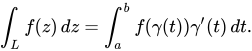
If the parametrization γ is continuously differentiable, the line integral can be evaluated as an integral of a function of a real variable: $${\displaystyle \int _{L}f(z)\,dz=\int _{a}^{b}f(\gamma (t))\gamma '(t)\,dt.}$$

When L is a closed curve (initial and final points coincide), the line integral is often denoted ${\textstyle \oint _{L}f(z)\,dz,}$ sometimes referred to in engineering as a cyclic integral.

To establish a complete analogy with the line integral of a vector field, one must go back to the definition of differentiability in multivariable calculus. The gradient is defined from Riesz representation theorem, and inner products in complex analysis involve conjugacy (the gradient of a function ${\displaystyle \gamma }$ at some ${\displaystyle z\in \mathbb {C} }$ would be ${\displaystyle {\overline {\gamma '(z)}}}$, and the complex inner product would attribute twice a conjugate to ${\displaystyle \gamma '}$ in the vector field definition of a line integral).

The line integral with respect to the conjugate complex differential ${\displaystyle {\overline {dz}}}$ is defined^[4] to be $${\displaystyle \int _{L}f(z){\overline {dz}}:={\overline {\int _{L}{\overline {f(z)}}\,dz}}=\int _{a}^{b}f(\gamma (t)){\overline {\gamma '(t)}}\,dt.}$$

The line integrals of complex functions can be evaluated using a number of techniques. The most direct is to split into real and imaginary parts, reducing the problem to evaluating two real-valued line integrals. The Cauchy integral theorem may be used to equate the line integral of an analytic function to the same integral over a more convenient curve. It also implies that over a closed curve enclosing a region where f(z) is analytic without singularities, the value of the integral is simply zero, or in case the region includes singularities, the residue theorem computes the integral in terms of the singularities. This also implies the path independence of complex line integral for analytic functions.

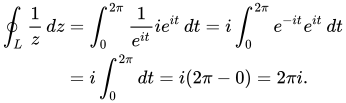
Consider the function f(z) = 1/z, and let the contour L be the counterclockwise unit circle about 0, parametrized by z(t) = e^it with t in [0, 2π] using the complex exponential. Substituting, we find: $${\displaystyle {\begin{aligned}\oint _{L}{\frac {1}{z}}\,dz&=\int _{0}^{2\pi }{\frac {1}{e^{it}}}ie^{it}\,dt=i\int _{0}^{2\pi }e^{-it}e^{it}\,dt\\&=i\int _{0}^{2\pi }dt=i(2\pi -0)=2\pi i.\end{aligned}}}$$

This is a typical result of Cauchy's integral formula and the residue theorem.

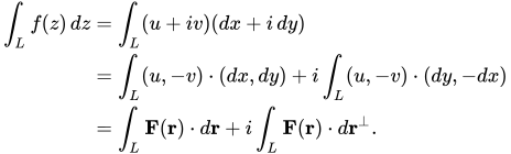
Viewing complex numbers as 2-dimensional vectors, the line integral of a complex-valued function ${\displaystyle f(z)}$ has real and complex parts equal to the line integral and the flux integral of the vector field corresponding to the conjugate function ${\displaystyle {\overline {f(z)}}.}$ Specifically, if ${\displaystyle \mathbf {r} (t)=(x(t),y(t))}$ parametrizes L, and ${\displaystyle f(z)=u(z)+iv(z)}$ corresponds to the vector field ${\displaystyle \mathbf {F} (x,y)={\overline {f(x+iy)}}=(u(x+iy),-v(x+iy)),}$ then: $${\displaystyle {\begin{aligned}\int _{L}f(z)\,dz&=\int _{L}(u+iv)(dx+i\,dy)\\&=\int _{L}(u,-v)\cdot (dx,dy)+i\int _{L}(u,-v)\cdot (dy,-dx)\\&=\int _{L}\mathbf {F} (\mathbf {r} )\cdot d\mathbf {r} +i\int _{L}\mathbf {F} (\mathbf {r} )\cdot d\mathbf {r} ^{\perp }.\end{aligned}}}$$

By Cauchy's theorem, the left-hand integral is zero when ${\displaystyle f(z)}$ is analytic (satisfying the Cauchy–Riemann equations) for any smooth closed curve L. Correspondingly, by Green's theorem, the right-hand integrals are zero when ${\displaystyle \mathbf {F} ={\overline {f(z)}}}$ is irrotational (curl-free) and incompressible (divergence-free). In fact, the Cauchy-Riemann equations for ${\displaystyle f(z)}$ are identical to the vanishing of curl and divergence for F.

By Green's theorem, the area of a region enclosed by a smooth, closed, positively oriented curve ${\displaystyle L}$ is given by the integral ${\textstyle {\frac {1}{2i}}\int _{L}{\overline {z}}\,dz.}$ This fact is used, for example, in the proof of the area theorem.

The path integral formulation of quantum mechanics actually refers not to path integrals in this sense but to functional integrals, that is, integrals over a space of paths, of a function of a possible path. However, path integrals in the sense of this article are important in quantum mechanics; for example, complex contour integration is often used in evaluating probability amplitudes in quantum scattering theory.

• "Integral over trajectories", Encyclopedia of Mathematics, EMS Press, 2001 [1994]
• Khan Academy modules:
  • "Introduction to the Line Integral"
  • "Line Integral Example 1"
  • "Line Integral Example 2 (part 1)"
  • "Line Integral Example 2 (part 2)"
• Path integral at PlanetMath.
• Line integral of a vector field – Interactive