Explore Black History

In the mathematical discipline of numerical linear algebra, a matrix splitting is an expression which represents a given matrix as a sum or difference of matrices. Many iterative methods (for example, for systems of differential equations) depend upon the direct solution of matrix equations involving matrices more general than tridiagonal matrices. These matrix equations can often be solved directly and efficiently when written as a matrix splitting. The technique was devised by Richard S. Varga in 1960.^[1]

We seek to solve the matrix equation

${\displaystyle \mathbf {A} \mathbf {x} =\mathbf {k} ,}$

1

where A is a given n × n non-singular matrix, and k is a given column vector with n components. We split the matrix A into

${\displaystyle \mathbf {A} =\mathbf {B} -\mathbf {C} ,}$

2

where B and C are n × n matrices. If, for an arbitrary n × n matrix M, M has nonnegative entries, we write M ≥ 0. If M has only positive entries, we write M > 0. Similarly, if the matrix M₁ − M₂ has nonnegative entries, we write M₁ ≥ M₂.

Definition: A = B − C is a regular splitting of A if B⁻¹ ≥ 0 and C ≥ 0.

We assume that matrix equations of the form

${\displaystyle \mathbf {B} \mathbf {x} =\mathbf {g} ,}$

3

where g is a given column vector, can be solved directly for the vector x. If (2) represents a regular splitting of A, then the iterative method

${\displaystyle \mathbf {B} \mathbf {x} ^{(m+1)}=\mathbf {C} \mathbf {x} ^{(m)}+\mathbf {k} ,\quad m=0,1,2,\ldots ,}$

4

where x⁽⁰⁾ is an arbitrary vector, can be carried out. Equivalently, we write (4) in the form

${\displaystyle \mathbf {x} ^{(m+1)}=\mathbf {B} ^{-1}\mathbf {C} \mathbf {x} ^{(m)}+\mathbf {B} ^{-1}\mathbf {k} ,\quad m=0,1,2,\ldots }$

5

The matrix D = B⁻¹C has nonnegative entries if (2) represents a regular splitting of A.^[2]

It can be shown that if A⁻¹ > 0, then ${\displaystyle \rho (\mathbf {D} )}$ < 1, where ${\displaystyle \rho (\mathbf {D} )}$ represents the spectral radius of D, and thus D is a convergent matrix. As a consequence, the iterative method (5) is necessarily convergent.^[3][4]

If, in addition, the splitting (2) is chosen so that the matrix B is a diagonal matrix (with the diagonal entries all non-zero, since B must be invertible), then B can be inverted in linear time (see Time complexity).

Many iterative methods can be described as a matrix splitting. If the diagonal entries of the matrix A are all nonzero, and we express the matrix A as the matrix sum

${\displaystyle \mathbf {A} =\mathbf {D} -\mathbf {U} -\mathbf {L} ,}$

6

where D is the diagonal part of A, and U and L are respectively strictly upper and lower triangular n × n matrices, then we have the following.

The Jacobi method can be represented in matrix form as a splitting

${\displaystyle \mathbf {x} ^{(m+1)}=\mathbf {D} ^{-1}(\mathbf {U} +\mathbf {L} )\mathbf {x} ^{(m)}+\mathbf {D} ^{-1}\mathbf {k} .}$[5][6]

7

The Gauss–Seidel method can be represented in matrix form as a splitting

${\displaystyle \mathbf {x} ^{(m+1)}=(\mathbf {D} -\mathbf {L} )^{-1}\mathbf {U} \mathbf {x} ^{(m)}+(\mathbf {D} -\mathbf {L} )^{-1}\mathbf {k} .}$[7][8]

8

The method of successive over-relaxation can be represented in matrix form as a splitting

${\displaystyle \mathbf {x} ^{(m+1)}=(\mathbf {D} -\omega \mathbf {L} )^{-1}[(1-\omega )\mathbf {D} +\omega \mathbf {U} ]\mathbf {x} ^{(m)}+\omega (\mathbf {D} -\omega \mathbf {L} )^{-1}\mathbf {k} .}$[9][10]

9

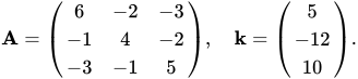
In equation (1), let

${\displaystyle \mathbf {A} ={\begin{pmatrix}6&-2&-3\\-1&4&-2\\-3&-1&5\end{pmatrix}},\quad \mathbf {k} ={\begin{pmatrix}5\\-12\\10\end{pmatrix}}.}$

10

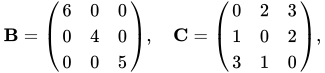
Let us apply the splitting (7) which is used in the Jacobi method: we split A in such a way that B consists of all of the diagonal elements of A, and C consists of all of the off-diagonal elements of A, negated. (Of course this is not the only useful way to split a matrix into two matrices.) We have

${\displaystyle {\begin{aligned}&\mathbf {B} ={\begin{pmatrix}6&0&0\\0&4&0\\0&0&5\end{pmatrix}},\quad \mathbf {C} ={\begin{pmatrix}0&2&3\\1&0&2\\3&1&0\end{pmatrix}},\end{aligned}}}$

11

${\displaystyle {\begin{aligned}&\mathbf {A^{-1}} ={\frac {1}{47}}{\begin{pmatrix}18&13&16\\11&21&15\\13&12&22\end{pmatrix}},\quad \mathbf {B^{-1}} ={\begin{pmatrix}{\frac {1}{6}}&0&0\\[4pt]0&{\frac {1}{4}}&0\\[4pt]0&0&{\frac {1}{5}}\end{pmatrix}},\end{aligned}}}$

${\displaystyle {\begin{aligned}\mathbf {D} =\mathbf {B^{-1}C} ={\begin{pmatrix}0&{\frac {1}{3}}&{\frac {1}{2}}\\[4pt]{\frac {1}{4}}&0&{\frac {1}{2}}\\[4pt]{\frac {3}{5}}&{\frac {1}{5}}&0\end{pmatrix}},\quad \mathbf {B^{-1}k} ={\begin{pmatrix}{\frac {5}{6}}\\[4pt]-3\\[4pt]2\end{pmatrix}}.\end{aligned}}}$

Since B⁻¹ ≥ 0 and C ≥ 0, the splitting (11) is a regular splitting. Since A⁻¹ > 0, the spectral radius ${\displaystyle \rho (\mathbf {D} )}$ < 1. (The approximate eigenvalues of D are ${\displaystyle \lambda _{i}\approx -0.4599820,-0.3397859,0.7997679.}$) Hence, the matrix D is convergent and the method (5) necessarily converges for the problem (10). Note that the diagonal elements of A are all greater than zero, the off-diagonal elements of A are all less than zero and A is strictly diagonally dominant.^[11]

The method (5) applied to the problem (10) then takes the form

${\displaystyle \mathbf {x} ^{(m+1)}={\begin{pmatrix}0&{\frac {1}{3}}&{\frac {1}{2}}\\[4pt]{\frac {1}{4}}&0&{\frac {1}{2}}\\[4pt]{\frac {3}{5}}&{\frac {1}{5}}&0\end{pmatrix}}\mathbf {x} ^{(m)}+{\begin{pmatrix}{\frac {5}{6}}\\[4pt]-3\\[4pt]2\end{pmatrix}},\quad m=0,1,2,\ldots }$

12

The exact solution to equation (12) is

${\displaystyle \mathbf {x} ={\begin{pmatrix}2\\-1\\3\end{pmatrix}}.}$

13

The first few iterates for equation (12) are listed in the table below, beginning with x⁽⁰⁾ = (0.0, 0.0, 0.0)^T. From the table one can see that the method is evidently converging to the solution (13), albeit rather slowly.

${\displaystyle x_{1}^{(m)}}$	${\displaystyle x_{2}^{(m)}}$	${\displaystyle x_{3}^{(m)}}$
0.0	0.0	0.0
0.83333	-3.0000	2.0000
0.83333	-1.7917	1.9000
1.1861	-1.8417	2.1417
1.2903	-1.6326	2.3433
1.4608	-1.5058	2.4477
1.5553	-1.4110	2.5753
1.6507	-1.3235	2.6510
1.7177	-1.2618	2.7257
1.7756	-1.2077	2.7783
1.8199	-1.1670	2.8238

As stated above, the Jacobi method (7) is the same as the specific regular splitting (11) demonstrated above.

Since the diagonal entries of the matrix A in problem (10) are all nonzero, we can express the matrix A as the splitting (6), where

${\displaystyle \mathbf {D} ={\begin{pmatrix}6&0&0\\0&4&0\\0&0&5\end{pmatrix}},\quad \mathbf {U} ={\begin{pmatrix}0&2&3\\0&0&2\\0&0&0\end{pmatrix}},\quad \mathbf {L} ={\begin{pmatrix}0&0&0\\1&0&0\\3&1&0\end{pmatrix}}.}$

14

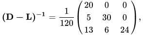
We then have

${\displaystyle {\begin{aligned}&\mathbf {(D-L)^{-1}} ={\frac {1}{120}}{\begin{pmatrix}20&0&0\\5&30&0\\13&6&24\end{pmatrix}},\end{aligned}}}$

${\displaystyle {\begin{aligned}&\mathbf {(D-L)^{-1}U} ={\frac {1}{120}}{\begin{pmatrix}0&40&60\\0&10&75\\0&26&51\end{pmatrix}},\quad \mathbf {(D-L)^{-1}k} ={\frac {1}{120}}{\begin{pmatrix}100\\-335\\233\end{pmatrix}}.\end{aligned}}}$

The Gauss–Seidel method (8) applied to the problem (10) takes the form

${\displaystyle \mathbf {x} ^{(m+1)}={\frac {1}{120}}{\begin{pmatrix}0&40&60\\0&10&75\\0&26&51\end{pmatrix}}\mathbf {x} ^{(m)}+{\frac {1}{120}}{\begin{pmatrix}100\\-335\\233\end{pmatrix}},\quad m=0,1,2,\ldots }$

15

The first few iterates for equation (15) are listed in the table below, beginning with x⁽⁰⁾ = (0.0, 0.0, 0.0)^T. From the table one can see that the method is evidently converging to the solution (13), somewhat faster than the Jacobi method described above.

${\displaystyle x_{1}^{(m)}}$	${\displaystyle x_{2}^{(m)}}$	${\displaystyle x_{3}^{(m)}}$
0.0	0.0	0.0
0.8333	-2.7917	1.9417
0.8736	-1.8107	2.1620
1.3108	-1.5913	2.4682
1.5370	-1.3817	2.6459
1.6957	-1.2531	2.7668
1.7990	-1.1668	2.8461
1.8675	-1.1101	2.8985
1.9126	-1.0726	2.9330
1.9423	-1.0479	2.9558
1.9619	-1.0316	2.9708

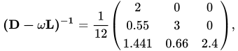
Let ω = 1.1. Using the splitting (14) of the matrix A in problem (10) for the successive over-relaxation method, we have

${\displaystyle {\begin{aligned}&\mathbf {(D-\omega L)^{-1}} ={\frac {1}{12}}{\begin{pmatrix}2&0&0\\0.55&3&0\\1.441&0.66&2.4\end{pmatrix}},\end{aligned}}}$

${\displaystyle {\begin{aligned}&\mathbf {(D-\omega L)^{-1}[(1-\omega )D+\omega U]} ={\frac {1}{12}}{\begin{pmatrix}-1.2&4.4&6.6\\-0.33&0.01&8.415\\-0.8646&2.9062&5.0073\end{pmatrix}},\end{aligned}}}$

${\displaystyle {\begin{aligned}&\mathbf {\omega (D-\omega L)^{-1}k} ={\frac {1}{12}}{\begin{pmatrix}11\\-36.575\\25.6135\end{pmatrix}}.\end{aligned}}}$

The successive over-relaxation method (9) applied to the problem (10) takes the form

${\displaystyle \mathbf {x} ^{(m+1)}={\frac {1}{12}}{\begin{pmatrix}-1.2&4.4&6.6\\-0.33&0.01&8.415\\-0.8646&2.9062&5.0073\end{pmatrix}}\mathbf {x} ^{(m)}+{\frac {1}{12}}{\begin{pmatrix}11\\-36.575\\25.6135\end{pmatrix}},\quad m=0,1,2,\ldots }$

16

The first few iterates for equation (16) are listed in the table below, beginning with x⁽⁰⁾ = (0.0, 0.0, 0.0)^T. From the table one can see that the method is evidently converging to the solution (13), slightly faster than the Gauss–Seidel method described above.

${\displaystyle x_{1}^{(m)}}$	${\displaystyle x_{2}^{(m)}}$	${\displaystyle x_{3}^{(m)}}$
0.0	0.0	0.0
0.9167	-3.0479	2.1345
0.8814	-1.5788	2.2209
1.4711	-1.5161	2.6153
1.6521	-1.2557	2.7526
1.8050	-1.1641	2.8599
1.8823	-1.0930	2.9158
1.9314	-1.0559	2.9508
1.9593	-1.0327	2.9709
1.9761	-1.0185	2.9829
1.9862	-1.0113	2.9901

• List of operator splitting topics
• Matrix decomposition
• M-matrix
• Stieltjes matrix

• Burden, Richard L.; Faires, J. Douglas (1993), Numerical Analysis (5th ed.), Boston: Prindle, Weber and Schmidt, ISBN 0-534-93219-3.
• Varga, Richard S. (1960). "Factorization and Normalized Iterative Methods". In Langer, Rudolph E. (ed.). Boundary Problems in Differential Equations. Madison: University of Wisconsin Press. pp. 121–142. LCCN 60-60003.
• Varga, Richard S. (1962), Matrix Iterative Analysis, New Jersey: Prentice-Hall, Bibcode:1962mia..book.....V, LCCN 62-21277.