Explore Black History

Mean shift is a non-parametric feature-space mathematical analysis technique for locating the maxima of a density function, a so-called mode-seeking algorithm.^[1] Application domains include cluster analysis in computer vision and image processing.^[2]

The mean shift procedure is usually credited to work by Fukunaga and Hostetler in 1975.^[3] It is, however, reminiscent of earlier work by Schnell in 1964.^[4]

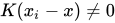
Mean shift is a procedure for locating the maxima—the modes—of a density function given discrete data sampled from that function.^[1] This is an iterative method, and we start with an initial estimate ${\displaystyle x}$. Let a kernel function ${\displaystyle K(x_{i}-x)}$ be given. This function determines the weight of nearby points for re-estimation of the mean. Typically a Gaussian kernel on the distance to the current estimate is used, ${\displaystyle K(x_{i}-x)=e^{-c||x_{i}-x||^{2}}}$. The weighted mean of the density in the window determined by ${\displaystyle K}$ is

${\displaystyle m(x)={\frac {\sum _{x_{i}\in N(x)}K(x_{i}-x)x_{i}}{\sum _{x_{i}\in N(x)}K(x_{i}-x)}}}$

where ${\displaystyle N(x)}$ is the neighborhood of ${\displaystyle x}$, a set of points for which ${\displaystyle K(x_{i}-x)\neq 0}$.

The difference ${\displaystyle m(x)-x}$ is called mean shift in Fukunaga and Hostetler.^[3] The mean-shift algorithm now sets ${\displaystyle x\leftarrow m(x)}$, and repeats the estimation until ${\displaystyle m(x)}$ converges.

Although the mean shift algorithm has been widely used in many applications, a rigid proof for the convergence of the algorithm using a general kernel in a high dimensional space is still not known.^[5] Aliyari Ghassabeh showed the convergence of the mean shift algorithm in one dimension with a differentiable, convex, and strictly decreasing profile function.^[6] However, the one-dimensional case has limited real world applications. Also, the convergence of the algorithm in higher dimensions with a finite number of the stationary (or isolated) points has been proved.^[5][7] However, sufficient conditions for a general kernel function to have finite stationary (or isolated) points have not been provided.

Gaussian Mean-Shift is an Expectation–maximization algorithm.^[8]

Let data be a finite set ${\displaystyle S}$ embedded in the ${\displaystyle n}$-dimensional Euclidean space, ${\displaystyle X}$. Let ${\displaystyle K}$ be a flat kernel that is the characteristic function of the ${\displaystyle \lambda }$-ball in ${\displaystyle X}$,

In each iteration of the algorithm, ${\displaystyle s\leftarrow m(s)}$ is performed for all ${\displaystyle s\in S}$ simultaneously. The first question, then, is how to estimate the density function given a sparse set of samples. One of the simplest approaches is to just smooth the data, e.g., by convolving it with a fixed kernel of width ${\displaystyle h}$,

where ${\displaystyle x_{i}}$ are the input samples and ${\displaystyle k(r)}$ is the kernel function (or Parzen window). ${\displaystyle h}$ is the only parameter in the algorithm and is called the bandwidth. This approach is known as kernel density estimation or the Parzen window technique. Once we have computed ${\displaystyle f(x)}$ from the equation above, we can find its local maxima using gradient ascent or some other optimization technique. The problem with this "brute force" approach is that, for higher dimensions, it becomes computationally prohibitive to evaluate ${\displaystyle f(x)}$ over the complete search space. Instead, mean shift uses a variant of what is known in the optimization literature as multiple restart gradient descent. Starting at some guess for a local maximum, ${\displaystyle y_{k}}$, which can be a random input data point ${\displaystyle x_{1}}$, mean shift computes the gradient of the density estimate ${\displaystyle f(x)}$ at ${\displaystyle y_{k}}$ and takes an uphill step in that direction.^[9]

Kernel definition: Let ${\displaystyle X}$ be the ${\displaystyle n}$-dimensional Euclidean space, ${\displaystyle \mathbb {R} ^{n}}$. The norm of ${\displaystyle x}$ is a non-negative number, ${\displaystyle \|x\|^{2}=x^{\top }x\geq 0}$. A function ${\displaystyle K:X\rightarrow \mathbb {R} }$ is said to be a kernel if there exists a profile, ${\displaystyle k:[0,\infty ]\rightarrow \mathbb {R} }$ , such that

${\displaystyle K(x)=k(\|x\|^{2})}$ and

• k is non-negative.
• k is non-increasing: ${\displaystyle k(a)\geq k(b)}$ if ${\displaystyle a<b}$.
• k is piecewise continuous and ${\displaystyle \int _{0}^{\infty }k(r)\,dr<\infty \ }$

The two most frequently used kernel profiles for mean shift are:

Flat kernel

Gaussian kernel

where the standard deviation parameter ${\displaystyle \sigma }$ works as the bandwidth parameter, ${\displaystyle h}$.

Consider a set of points in two-dimensional space. Assume a circular window centered at ${\displaystyle C}$ and having radius ${\displaystyle r}$ as the kernel. Mean-shift is a hill climbing algorithm which involves shifting this kernel iteratively to a higher density region until convergence. Every shift is defined by a mean shift vector. The mean shift vector always points toward the direction of the maximum increase in the density. At every iteration the kernel is shifted to the centroid or the mean of the points within it. The method of calculating this mean depends on the choice of the kernel. In this case if a Gaussian kernel is chosen instead of a flat kernel, then every point will first be assigned a weight which will decay exponentially as the distance from the kernel's center increases. At convergence, there will be no direction at which a shift can accommodate more points inside the kernel.

The mean shift algorithm can be used for visual tracking. The simplest such algorithm would create a confidence map in the new image based on the color histogram of the object in the previous image, and use mean shift to find the peak of a confidence map near the object's old position. The confidence map is a probability density function on the new image, assigning each pixel of the new image a probability, which is the probability of the pixel color occurring in the object in the previous image. A few algorithms, such as kernel-based object tracking,^[10] ensemble tracking,^[11] CAMshift ^[12][13] expand on this idea.

Let ${\displaystyle x_{i}}$ and ${\displaystyle z_{i},i=1,...,n,}$ be the ${\displaystyle d}$-dimensional input and filtered image pixels in the joint spatial-range domain. For each pixel,

• Initialize ${\displaystyle j=1}$ and ${\displaystyle y_{i,1}=x_{i}}$
• Compute ${\displaystyle y_{i,j+1}}$ according to ${\displaystyle m(\cdot )}$ until convergence, ${\displaystyle y=y_{i,c}}$.
• Assign ${\displaystyle z_{i}=(x_{i}^{s},y_{i,c}^{r})}$. The superscripts s and r denote the spatial and range components of a vector, respectively. The assignment specifies that the filtered data at the spatial location axis will have the range component of the point of convergence ${\displaystyle y_{i,c}^{r}}$.

1. Mean shift is an application-independent tool suitable for real data analysis.
2. Does not assume any predefined shape on data clusters.
3. It is capable of handling arbitrary feature spaces.
4. The procedure relies on choice of a single parameter: bandwidth.
5. The bandwidth/window size 'h' has a physical meaning, unlike k-means.

1. The selection of a window size is not trivial.
2. Inappropriate window size can cause modes to be merged, or generate additional "shallow" modes.
3. Often requires using adaptive window size.

Variants of the algorithm can be found in machine learning and image processing packages:

• ELKI. Java data mining tool with many clustering algorithms.
• ImageJ. Image filtering using the mean shift filter.
• mlpack. Efficient dual-tree algorithm-based implementation.
• OpenCV contains mean-shift implementation via cvMeanShift Method
• Orfeo toolbox. A C++ implementation.
• scikit-learn Numpy/Python implementation uses ball tree for efficient neighboring points lookup

• DBSCAN
• OPTICS algorithm
• Kernel density estimation (KDE)
• Kernel (statistics)