Explore Black History

A negative-feedback amplifier (or feedback amplifier) is an electronic amplifier that subtracts a fraction of its output from its input, so that negative feedback opposes the original signal.^[1] The applied negative feedback can improve its performance (gain stability, linearity, frequency response, step response) and reduces sensitivity to parameter variations due to manufacturing or environment. Because of these advantages, many amplifiers and control systems use negative feedback.^[2]

An idealized negative-feedback amplifier as shown in the diagram is a system of three elements (see Figure 1):

• an amplifier with gain A_OL,
• a feedback network β, which senses the output signal and possibly transforms it in some way (for example by attenuating or filtering it),
• a summing circuit that acts as a subtractor (the circle in the figure), which combines the input and the transformed output.

Fundamentally, all electronic devices that provide power gain (e.g., vacuum tubes, bipolar transistors, MOS transistors) are nonlinear. Negative feedback trades gain for higher linearity (reducing distortion) and can provide other benefits. If not designed correctly, amplifiers with negative feedback can under some circumstances become unstable due to the feedback becoming positive, resulting in unwanted behavior such as oscillation. The Nyquist stability criterion developed by Harry Nyquist of Bell Laboratories is used to study the stability of feedback amplifiers.

Feedback amplifiers share these properties:^[3]

Pros:

• Can increase or decrease input impedance (depending on type of feedback).
• Can increase or decrease output impedance (depending on type of feedback).
• Reduces total distortion if sufficiently applied (increases linearity).
• Increases the bandwidth.
• Desensitizes gain to component variations.
• Can control step response of amplifier.

Cons:

• May lead to instability if not designed carefully.
• Amplifier gain decreases.
• Input and output impedances of a negative-feedback amplifier (closed-loop amplifier) become sensitive to the gain of an amplifier without feedback (open-loop amplifier)—that exposes these impedances to variations in the open-loop gain, for example, due to parameter variations or nonlinearity of the open-loop gain.
• Changes the composition of the distortion (increasing audibility) if insufficiently applied.

Paul Voigt patented a negative feedback amplifier in January 1924, though his theory lacked detail.^[4] Harold Stephen Black independently invented the negative-feedback amplifier while he was a passenger on the Lackawanna Ferry (from Hoboken Terminal to Manhattan) on his way to work at Bell Laboratories (located in Manhattan instead of New Jersey in 1927) on August 6th, 1927^[5] (US Patent 2,102,671,^[6] issued in 1937). Black was working on reducing distortion in repeater amplifiers used for telephone transmission. On a blank space in his copy of The New York Times,^[7] he recorded the diagram found in Figure 1 and the equations derived below.^[8] On August 8, 1928, Black submitted his invention to the U. S. Patent Office, which took more than 9 years to issue the patent. Black later wrote: "One reason for the delay was that the concept was so contrary to established beliefs that the Patent Office initially did not believe it would work."^[9]

Using the model of two unilateral blocks, several consequences of feedback are simply derived.

Below, the voltage gain of the amplifier with feedback, the closed-loop gain A_FB, is derived in terms of the gain of the amplifier without feedback, the open-loop gain A_OL and the feedback factor β, which governs how much of the output signal is applied to the input (see Figure 1). The open-loop gain A_OL in general may be a function of both frequency and voltage; the feedback parameter β is determined by the feedback network that is connected around the amplifier. For an operational amplifier, two resistors forming a voltage divider may be used for the feedback network to set β between 0 and 1. This network may be modified using reactive elements like capacitors or inductors to (a) give frequency-dependent closed-loop gain as in equalization/tone-control circuits or (b) construct oscillators. The gain of the amplifier with feedback is derived below in the case of a voltage amplifier with voltage feedback.

Without feedback, the input voltage V′_in is applied directly to the amplifier input. The according output voltage is

${\displaystyle V_{\text{out}}=A_{\text{OL}}\cdot V'_{\text{in}}.}$

Suppose now that an attenuating feedback loop applies a fraction ${\displaystyle \beta \cdot V_{\text{out}}}$ of the output to one of the subtractor inputs so that it subtracts from the circuit input voltage V_in applied to the other subtractor input. The result of subtraction applied to the amplifier input is

${\displaystyle V'_{\text{in}}=V_{\text{in}}-\beta \cdot V_{\text{out}}.}$

Substituting for V′_in in the first expression,

${\displaystyle V_{\text{out}}=A_{\text{OL}}(V_{\text{in}}-\beta \cdot V_{\text{out}}).}$

Rearranging:

${\displaystyle V_{\text{out}}(1+\beta \cdot A_{\text{OL}})=V_{\text{in}}\cdot A_{\text{OL}}.}$

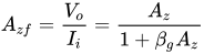
Then the gain of the amplifier with feedback, called the closed-loop gain, A_FB is given by

${\displaystyle A_{\text{FB}}={\frac {V_{\text{out}}}{V_{\text{in}}}}={\frac {A_{\text{OL}}}{1+\beta \cdot A_{\text{OL}}}}.}$

If A_OL ≫ 1, then A_FB ≈ 1 / β, and the effective amplification (or closed-loop gain) A_FB is set by the feedback constant β, and hence set by the feedback network, usually a simple reproducible network, thus making linearizing and stabilizing the amplification characteristics straightforward. If there are conditions where β A_OL = −1, the amplifier has infinite amplification – it has become an oscillator, and the system is unstable. The stability characteristics of the gain feedback product β A_OL are often displayed and investigated on a Nyquist plot (a polar plot of the gain/phase shift as a parametric function of frequency). A simpler, but less general technique, uses Bode plots.

The combination L = −β A_OL appears commonly in feedback analysis and is called the loop gain. The combination (1 + β A_OL) also appears commonly and is variously named as the desensitivity factor, return difference, or improvement factor.^[10]

• Open-loop gain = ${\displaystyle A_{\text{OL}}}$^{[11][12][13][14]}
• Closed-loop gain = ${\displaystyle {\frac {A_{\text{OL}}}{1+\beta \cdot A_{\text{OL}}}}}$
• Feedback factor = ${\displaystyle \beta }$
• Noise gain = ${\displaystyle 1/\beta }$^{[dubious – discuss]}
• Loop gain = ${\displaystyle -\beta \cdot A_{\text{OL}}}$
• Desensitivity factor = ${\displaystyle 1+\beta \cdot A_{\text{OL}}}$

Feedback can be used to extend the bandwidth of an amplifier at the cost of lowering the amplifier gain.^[15] Figure 2 shows such a comparison. The figure is understood as follows. Without feedback the so-called open-loop gain in this example has a single-time-constant frequency response given by

${\displaystyle A_{\text{OL}}(f)={\frac {A_{0}}{1+jf/f_{\text{C}}}},}$

where f_C is the cutoff or corner frequency of the amplifier: in this example f_C = 10⁴ Hz, and the gain at zero frequency A₀ = 10⁵ V/V. The figure shows that the gain is flat out to the corner frequency and then drops. When feedback is present, the so-called closed-loop gain, as shown in the formula of the previous section, becomes

${\displaystyle {\begin{aligned}A_{\text{FB}}(f)&={\frac {A_{\text{OL}}}{1+\beta A_{\text{OL}}}}\\&={\frac {A_{0}/(1+jf/f_{\text{C}})}{1+\beta A_{0}/(1+jf/f_{\text{C}})}}\\&={\frac {A_{0}}{1+jf/f_{\text{C}}+\beta A_{0}}}\\&={\frac {A_{0}}{(1+\beta A_{0})\left(1+j{\frac {f}{(1+\beta A_{0})f_{\text{C}}}}\right)}}.\end{aligned}}}$

The last expression shows that the feedback amplifier still has a single-time-constant behavior, but the corner frequency is now increased by the improvement factor (1 + β A₀), and the gain at zero frequency has dropped by exactly the same factor. This behavior is called the gain–bandwidth tradeoff. In Figure 2, (1 + β A₀) = 10³, so A_FB(0) = 10⁵ / 10³ = 100 V/V, and f_C increases to 10⁴ × 10³ = 10⁷ Hz.

When the close-loop gain has several poles, rather than the single pole of the above example, feedback can result in complex poles (real and imaginary parts). In a two-pole case, the result is peaking in the frequency response of the feedback amplifier near its corner frequency and ringing and overshoot in its step response. In the case of more than two poles, the feedback amplifier can become unstable and oscillate. See the discussion of gain margin and phase margin. For a complete discussion, see Sansen.^[16]

A principal idealization behind the formulation of the Introduction is the network's division into two autonomous blocks (that is, with their own individually determined transfer functions), a simple example of what often is called "circuit partitioning",^[17] which refers in this instance to the division into a forward amplification block and a feedback block. In practical amplifiers, the information flow is not unidirectional as shown here.^[18] Frequently these blocks are taken to be two-port networks to allow inclusion of bilateral information transfer.^[19][20] Casting an amplifier into this form is a non-trivial task, however, especially when the feedback involved is not global (that is directly from the output to the input) but local (that is, feedback within the network, involving nodes that do not coincide with input and/or output terminals).^[21][22]

In these more general cases, the amplifier is analyzed more directly without the partitioning into blocks like those in the diagram, using instead some analysis based upon signal-flow analysis, such as the return-ratio method or the asymptotic gain model.^[24][25][26] Commenting upon the signal-flow approach, Choma says:^[27]

"In contrast to block diagram and two-port approaches to the feedback network analysis problem, signal flow methods mandate no a priori assumptions as to the unilateral or bilateral properties of the open loop and feedback subcircuits. Moreover, they are not predicated on mutually independent open loop and feedback subcircuit transfer functions, and they do not require that feedback be implemented only globally. Indeed signal flow techniques do not even require explicit identification of the open loop and feedback subcircuits. Signal flow thus removes the detriments pervasive of conventional feedback network analyses but additionally, it proves to be computationally efficient as well."

Following up on this suggestion, a signal-flow graph for a negative-feedback amplifier is shown in the figure, which is patterned after one by D'Amico et al..^[23] Following these authors, the notation is as follows:

"Variables x_S, x_O represent the input and output signals, moreover, two other generic variables, x_i, x_j linked together through the control (or critical) parameter P are explicitly shown. Parameters a_ij are the weight branches. Variables x_i, x_j and the control parameter, P, model a controlled generator, or the relation between voltage and current across two nodes of the circuit.

The term a₁₁ is the transfer function between the input and the output [after] setting the control parameter, P, to zero; term a₁₂ is the transfer function between the output and the controlled variable x_j [after] setting the input source, x_S, to zero; term a₂₁ represents the transfer function between the source variable and the inner variable, x_i when the controlled variable x_j is set to zero (i.e., when the control parameter, P is set to zero); term a₂₂ gives the relation between the independent and the controlled inner variables setting control parameter, P and input variable, x_S, to zero."

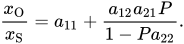
Using this graph, these authors derive the generalized gain expression in terms of the control parameter P that defines the controlled source relationship x_j = Px_i:

${\displaystyle x_{\text{O}}=a_{11}x_{\text{S}}+a_{12}x_{j},}$

${\displaystyle x_{i}=a_{21}x_{\text{S}}+a_{22}x_{j},}$

${\displaystyle x_{j}=Px_{i}.}$

Combining these results, the gain is given by

${\displaystyle {\frac {x_{\text{O}}}{x_{\text{S}}}}=a_{11}+{\frac {a_{12}a_{21}P}{1-Pa_{22}}}.}$

To employ this formula, one has to identify a critical controlled source for the particular amplifier circuit in hand. For example, P could be the control parameter of one of the controlled sources in a two-port network, as shown for a particular case in D'Amico et al.^[23] As a different example, if we take a₁₂ = a₂₁ = 1, P = A, a₂₂ = –β (negative feedback) and a₁₁ = 0 (no feedforward), we regain the simple result with two unidirectional blocks.

Although, as mentioned in the section Signal-flow analysis, some form of signal-flow analysis is the most general way to treat the negative-feedback amplifier, representation as two two-ports is the approach most often presented in textbooks and is presented here. It retains a two-block circuit partition of the amplifier, but allows the blocks to be bilateral. Some drawbacks of this method are described at the end.

Electronic amplifiers use current or voltage as input and output, so four types of amplifier are possible (any of two possible inputs with any of two possible outputs). See classification of amplifiers. The objective for the feedback amplifier may be any one of the four types of amplifier and is not necessarily the same type as the open-loop amplifier, which itself may be any one of these types. So, for example, an op amp (voltage amplifier) can be arranged to make a current amplifier instead.

Negative-feedback amplifiers of any type can be implemented using combinations of two-port networks. There are four types of two-port network, and the type of amplifier desired dictates the choice of two-ports and the selection of one of the four different connection topologies shown in the diagram. These connections are usually referred to as series or shunt (parallel) connections.^[29][30] In the diagram, the left column shows shunt inputs; the right column shows series inputs. The top row shows series outputs; the bottom row shows shunt outputs. The various combinations of connections and two-ports are listed in the table below.

For example, for a current-feedback amplifier, current from the output is sampled for feedback and combined with current at the input. Therefore, the feedback ideally is performed using an (output) current-controlled current source (CCCS), and its imperfect realization using a two-port network also must incorporate a CCCS, that is, the appropriate choice for feedback network is a g-parameter two-port. Here the two-port method used in most textbooks is presented,^{[31][32][33][34]} using the circuit treated in the article on asymptotic gain model.

Figure 3 shows a two-transistor amplifier with a feedback resistor R_f. The aim is to analyze this circuit to find three items: the gain, the output impedance looking into the amplifier from the load, and the input impedance looking into the amplifier from the source.

The first step is replacement of the feedback network by a two-port. Just what components go into the two-port?

On the input side of the two-port we have R_f. If the voltage at the right side of R_f changes, it changes the current in R_f that is subtracted from the current entering the base of the input transistor. That is, the input side of the two-port is a dependent current source controlled by the voltage at the top of resistor R₂.

One might say the second stage of the amplifier is just a voltage follower, transmitting the voltage at the collector of the input transistor to the top of R₂. That is, the monitored output signal is really the voltage at the collector of the input transistor. That view is legitimate, but then the voltage follower stage becomes part of the feedback network. That makes analysis of feedback more complicated.

An alternative view is that the voltage at the top of R₂ is set by the emitter current of the output transistor. That view leads to an entirely passive feedback network made up of R₂ and R_f. The variable controlling the feedback is the emitter current, so the feedback is a current-controlled current source (CCCS). We search through the four available two-port networks and find the only one with a CCCS is the g-parameter two-port, shown in Figure 4. The next task is to select the g-parameters so that the two-port of Figure 4 is electrically equivalent to the L-section made up of R₂ and R_f. That selection is an algebraic procedure made most simply by looking at two individual cases: the case with V₁ = 0, which makes the VCVS on the right side of the two-port a short-circuit; and the case with I₂ = 0. which makes the CCCS on the left side an open circuit. The algebra in these two cases is simple, much easier than solving for all variables at once. The choice of g-parameters that make the two-port and the L-section behave the same way are shown in the table below.

g11	g12	g21	g22
${\displaystyle {\frac {1}{R_{\mathrm {f} }+R_{2}}}}$	${\displaystyle -{\frac {R_{2}}{R_{2}+R_{\mathrm {f} }}}}$	${\displaystyle {\frac {R_{2}}{R_{2}+R_{\mathrm {f} }}}}$	${\displaystyle R_{2}||R_{\mathrm {f} }\ }$

The next step is to draw the small-signal schematic for the amplifier with the two-port in place using the hybrid-pi model for the transistors. Figure 5 shows the schematic with notation R₃ = R_C2 || R_L and R₁₁ = 1 / g₁₁, R₂₂ = g₂₂.

Figure 3 indicates the output node, but not the choice of output variable. A useful choice is the short-circuit current output of the amplifier (leading to the short-circuit current gain). Because this variable leads simply to any of the other choices (for example, load voltage or load current), the short-circuit current gain is found below.

First the loaded open-loop gain is found. The feedback is turned off by setting g₁₂ = g₂₁ = 0. The idea is to find how much the amplifier gain is changed because of the resistors in the feedback network by themselves, with the feedback turned off. This calculation is pretty easy because R₁₁, R_B, and r_π1 all are in parallel and v₁ = v_π. Let R₁ = R₁₁ || R_B || r_π1. In addition, i₂ = −(β+1) i_B. The result for the open-loop current gain A_OL is:

${\displaystyle A_{\mathrm {OL} }={\frac {\beta i_{\mathrm {B} }}{i_{\mathrm {S} }}}=g_{m}R_{\mathrm {C} }\left({\frac {\beta }{\beta +1}}\right)\left({\frac {R_{1}}{R_{22}+{\frac {r_{\pi 2}+R_{\mathrm {C} }}{\beta +1}}}}\right)\ .}$

In the classical approach to feedback, the feedforward represented by the VCVS (that is, g₂₁ v₁) is neglected.^[35] That makes the circuit of Figure 5 resemble the block diagram of Figure 1, and the gain with feedback is then:

${\displaystyle A_{\mathrm {FB} }={\frac {A_{\mathrm {OL} }}{1+{\beta }_{\mathrm {FB} }A_{\mathrm {OL} }}}}$

${\displaystyle A_{\mathrm {FB} }={\frac {A_{\mathrm {OL} }}{1+{\frac {R_{2}}{R_{2}+R_{\mathrm {f} }}}A_{\mathrm {OL} }}}\ ,}$

where the feedback factor β_FB = −g₁₂. Notation β_FB is introduced for the feedback factor to distinguish it from the transistor β.

Feedback is used to better match signal sources to their loads. For example, a direct connection of a voltage source to a resistive load may result in signal loss due to voltage division, but interjecting a negative feedback amplifier can increase the apparent load seen by the source, and reduce the apparent driver impedance seen by the load, avoiding signal attenuation by voltage division. This advantage is not restricted to voltage amplifiers, but analogous improvements in matching can be arranged for current amplifiers, transconductance amplifiers and transresistance amplifiers.

To explain these effects of feedback upon impedances, first a digression on how two-port theory approaches resistance determination, and then its application to the amplifier at hand.

Figure 6 shows an equivalent circuit for finding the input resistance of a feedback voltage amplifier (left) and for a feedback current amplifier (right). These arrangements are typical Miller theorem applications.

In the case of the voltage amplifier, the output voltage βV_out of the feedback network is applied in series and with an opposite polarity to the input voltage V_x travelling over the loop (but in respect to ground, the polarities are the same). As a result, the effective voltage across and the current through the amplifier input resistance R_in decrease so that the circuit input resistance increases (one might say that R_in apparently increases). Its new value can be calculated by applying Miller theorem (for voltages) or the basic circuit laws. Thus Kirchhoff's voltage law provides:

${\displaystyle V_{x}=I_{x}R_{\mathrm {in} }+\beta v_{\mathrm {out} }\ ,}$

where v_out = A_v v_in = A_v I_x R_in. Substituting this result in the above equation and solving for the input resistance of the feedback amplifier, the result is:

${\displaystyle R_{\mathrm {in} }(fb)={\frac {V_{x}}{I_{x}}}=\left(1+\beta A_{v}\right)R_{\mathrm {in} }\ .}$

The general conclusion from this example and a similar example for the output resistance case is: A series feedback connection at the input (output) increases the input (output) resistance by a factor ( 1 + β A_OL ), where A_OL = open loop gain.

On the other hand, for the current amplifier, the output current βI_out of the feedback network is applied in parallel and with an opposite direction to the input current I_x. As a result, the total current flowing through the circuit input (not only through the input resistance R_in) increases and the voltage across it decreases so that the circuit input resistance decreases (R_in apparently decreases). Its new value can be calculated by applying the dual Miller theorem (for currents) or the basic Kirchhoff's laws:

${\displaystyle I_{x}={\frac {V_{\mathrm {in} }}{R_{\mathrm {in} }}}+\beta i_{\mathrm {out} }\ .}$

where i_out = A_i i_in = A_i V_x / R_in. Substituting this result in the above equation and solving for the input resistance of the feedback amplifier, the result is:

${\displaystyle R_{\mathrm {in} }(fb)={\frac {V_{x}}{I_{x}}}={\frac {R_{\mathrm {in} }}{\left(1+\beta A_{i}\right)}}\ .}$

The general conclusion from this example and a similar example for the output resistance case is: A parallel feedback connection at the input (output) decreases the input (output) resistance by a factor ( 1 + β A_OL ), where A_OL = open loop gain.

These conclusions can be generalized to treat cases with arbitrary Norton or Thévenin drives, arbitrary loads, and general two-port feedback networks. However, the results do depend upon the main amplifier having a representation as a two-port – that is, the results depend on the same current entering and leaving the input terminals, and likewise, the same current that leaves one output terminal must enter the other output terminal.

A broader conclusion, independent of the quantitative details, is that feedback can be used to increase or to decrease the input and output impedance.

These resistance results now are applied to the amplifier of Figure 3 and Figure 5. The improvement factor that reduces the gain, namely ( 1 + β_FB A_OL), directly decides the effect of feedback upon the input and output resistances of the amplifier. In the case of a shunt connection, the input impedance is reduced by this factor; and in the case of series connection, the impedance is multiplied by this factor. However, the impedance that is modified by feedback is the impedance of the amplifier in Figure 5 with the feedback turned off, and does include the modifications to impedance caused by the resistors of the feedback network.

Therefore, the input impedance seen by the source with feedback turned off is R_in = R₁ = R₁₁ || R_B || r_π1, and with the feedback turned on (but no feedforward)

${\displaystyle R_{\mathrm {in} }={\frac {R_{1}}{1+{\beta }_{\mathrm {FB} }A_{\mathrm {OL} }}}\ ,}$

where division is used because the input connection is shunt: the feedback two-port is in parallel with the signal source at the input side of the amplifier. A reminder: A_OL is the loaded open loop gain found above, as modified by the resistors of the feedback network.

The impedance seen by the load needs further discussion. The load in Figure 5 is connected to the collector of the output transistor, and therefore is separated from the body of the amplifier by the infinite impedance of the output current source. Therefore, feedback has no effect on the output impedance, which remains simply R_C2 as seen by the load resistor R_L in Figure 3.^[36][37]

If instead we wanted to find the impedance presented at the emitter of the output transistor (instead of its collector), which is series connected to the feedback network, feedback would increase this resistance by the improvement factor ( 1 + β_FB A_OL).^[38]

The gain derived above is the current gain at the collector of the output transistor. To relate this gain to the gain when voltage is the output of the amplifier, notice that the output voltage at the load R_L is related to the collector current by Ohm's law as v_L = i_C (R_C2 || R_L). Consequently, the transresistance gain v_L / i_S is found by multiplying the current gain by R_C2 || R_L:

${\displaystyle {\frac {v_{\mathrm {L} }}{i_{\mathrm {S} }}}=A_{\mathrm {FB} }(R_{\mathrm {C2} }\parallel R_{\mathrm {L} })\ .}$

Similarly, if the output of the amplifier is taken to be the current in the load resistor R_L, current division determines the load current, and the gain is then:

${\displaystyle {\frac {i_{\mathrm {L} }}{i_{\mathrm {S} }}}=A_{\mathrm {FB} }{\frac {R_{\mathrm {C2} }}{R_{\mathrm {C2} }+R_{\mathrm {L} }}}\ .}$

Some drawbacks of the two two-port approach follow, intended for the attentive reader.

Figure 7 shows the small-signal schematic with the main amplifier and the feedback two-port in shaded boxes. The feedback two-port satisfies the port conditions: at the input port, I_in enters and leaves the port, and likewise at the output, I_out enters and leaves.

Is the main amplifier block also a two-port? The main amplifier is shown in the upper shaded box. The ground connections are labeled. Figure 7 shows the interesting fact that the main amplifier does not satisfy the port conditions at its input and output unless the ground connections are chosen to make that happen. For example, on the input side, the current entering the main amplifier is I_S. This current is divided three ways: to the feedback network, to the bias resistor R_B and to the base resistance of the input transistor r_π. To satisfy the port condition for the main amplifier, all three components must be returned to the input side of the main amplifier, which means all the ground leads labeled G₁ must be connected, as well as emitter lead G_E1. Likewise, on the output side, all ground connections G₂ must be connected and also ground connection G_E2. Then, at the bottom of the schematic, underneath the feedback two-port and outside the amplifier blocks, G₁ is connected to G₂. That forces the ground currents to divide between the input and output sides as planned. Notice that this connection arrangement splits the emitter of the input transistor into a base-side and a collector-side – a physically impossible thing to do, but electrically the circuit sees all the ground connections as one node, so this fiction is permitted.

Of course, the way the ground leads are connected makes no difference to the amplifier (they are all one node), but it makes a difference to the port conditions. This artificiality is a weakness of this approach: the port conditions are needed to justify the method, but the circuit really is unaffected by how currents are traded among ground connections.

However, if no possible arrangement of ground conditions leads to the port conditions, the circuit might not behave the same way.^[39] The improvement factors (1 + β_FB A_OL) for determining input and output impedance might not work.^[40] This situation is awkward, because a failure to make a two-port may reflect a real problem (it just is not possible), or reflect a lack of imagination (for example, just did not think of splitting the emitter node in two). As a consequence, when the port conditions are in doubt, at least two approaches are possible to establish whether improvement factors are accurate: either simulate an example using Spice and compare results with use of an improvement factor, or calculate the impedance using a test source and compare results.

A more practical choice is to drop the two-port approach altogether, and use various alternatives based on signal flow graph theory, including the Rosenstark method, the Choma method, and use of Blackman's theorem.^[41] That choice may be advisable if small-signal device models are complex, or are not available (for example, the devices are known only numerically, perhaps from measurement or from SPICE simulations).

Summarizing the two-port analysis of feedback, one can get this table of formulas.^[34]

Feedback Amplifier	Source Signal	Output Signal	Transfer Function	Input Resistance	Output Resistance
Series-Shunt (voltage amplifier)	Voltage	Voltage	${\displaystyle A_{vf}={\frac {V_{o}}{V_{i}}}={\frac {A_{v}}{1+\beta _{v}A_{v}}}}$	${\displaystyle R_{i}(1+\beta _{v}A_{v})}$	${\displaystyle {\frac {R_{o}}{1+\beta _{v}A_{v}}}}$
Shunt-Series (current amplifier)	Current	Current	${\displaystyle A_{if}={\frac {I_{o}}{I_{i}}}={\frac {A_{i}}{1+\beta _{i}A_{i}}}}$	${\displaystyle {\frac {R_{i}}{1+\beta _{i}A_{i}}}}$	${\displaystyle R_{o}(1+\beta _{i}A_{i})}$
Series-Series(transconductance amplifier)	Voltage	Current	${\displaystyle A_{gf}={\frac {I_{o}}{V_{i}}}={\frac {A_{g}}{1+\beta _{z}A_{g}}}}$	${\displaystyle R_{i}(1+\beta _{z}A_{g})}$	${\displaystyle R_{o}(1+\beta _{z}A_{g})}$
Shunt-Shunt (transresistance amplifier)	Current	Voltage	${\displaystyle A_{zf}={\frac {V_{o}}{I_{i}}}={\frac {A_{z}}{1+\beta _{g}A_{z}}}}$	${\displaystyle {\frac {R_{i}}{1+\beta _{g}A_{z}}}}$	${\displaystyle {\frac {R_{o}}{1+\beta _{g}A_{z}}}}$

The variables and their meanings are

${\displaystyle A}$- gain, ${\displaystyle I}$- current, ${\displaystyle V}$- voltage,${\displaystyle \beta }$- feedback gain and ${\displaystyle R}$- resistance.

The subscripts and their meanings are

${\displaystyle f}$- feedback amplifier, ${\displaystyle v}$- voltage,${\displaystyle g}$- transconductance, ${\displaystyle Z}$- transresistance, ${\displaystyle o}$- output and ${\displaystyle i}$- current for gains and feedback and ${\displaystyle i}$- input for resistances.

For example ${\displaystyle A_{vf}}$means voltage feedback amplifier gain.^[34]

Simple amplifiers like the common emitter configuration have primarily low-order distortion, such as the 2nd and 3rd harmonics. In audio systems, these can be minimally audible because musical signals are typically already a harmonic series, and the low-order distortion products are hidden by the masking effect of the human hearing system.^[42][43]

After applying moderate amounts of negative feedback (10–15 dB), the low-order harmonics are reduced, but higher-order harmonics are introduced.^[44] Since these are not masked as well, the distortion becomes audibly worse, even though the overall THD may go down.^[44] This has led to a persistent myth that negative feedback is detrimental in audio amplifiers,^[45] leading audiophile manufacturers to market their amplifiers as "zero feedback" (even when they use local feedback to linearize each stage).^[46][47]

However, as the amount of negative feedback is increased further, all harmonics are reduced, returning the distortion to inaudibility, and then improving it beyond the original zero-feedback stage (provided the system is strictly stable).^[48][45][49] So the problem is not negative feedback, but insufficient amounts of it.

• Asymptotic gain model
• Blackman's theorem
• Bode plot
• Buffer amplifier considers the basic op-amp amplifying stage with negative feedback
• Common collector (emitter follower) is dedicated to the basic transistor amplifying stage with negative feedback
• Extra element theorem
• Frequency compensation
• Miller theorem is a powerful tool for determining the input/output impedances of negative feedback circuits
• Operational amplifier presents the basic op-amp non-inverting amplifier and inverting amplifier
• Operational amplifier applications shows the most typical op-amp circuits with negative feedback
• Phase margin
• Pole splitting
• Return ratio
• Step response