Explore Black History

Notation	${\displaystyle {\textrm {NM}}(x_{0},\,\mathbf {p} )}$
Parameters	${\displaystyle x_{0}>0}$ — the number of failures before the experiment is stopped, ${\displaystyle \mathbf {p} }$ ∈ Rm — m-vector of "success" probabilities, p0 = 1 − (p1+…+pm) — the probability of a "failure".
Support	${\displaystyle x_{i}\in \{0,1,2,\ldots \},1\leq i\leq m}$
PMF	${\displaystyle \Gamma \!\left(\sum _{i=0}^{m}{x_{i}}\right){\frac {p_{0}^{x_{0}}}{\Gamma (x_{0})}}\prod _{i=1}^{m}{\frac {p_{i}^{x_{i}}}{x_{i}!}},}$ where Γ(x) is the Gamma function.
Mean	${\displaystyle {\tfrac {x_{0}}{p_{0}}}\,\mathbf {p} }$
Variance	${\displaystyle {\tfrac {x_{0}}{p_{0}^{2}}}\,\mathbf {pp} '+{\tfrac {x_{0}}{p_{0}}}\,\operatorname {diag} (\mathbf {p} )}$
MGF	${\displaystyle {\bigg (}{\frac {p_{0}}{1-\sum _{j=1}^{m}p_{j}e^{t_{j}}}}{\bigg )}^{\!x_{0}}}$
CF	${\displaystyle {\bigg (}{\frac {p_{0}}{1-\sum _{j=1}^{m}p_{j}e^{it_{j}}}}{\bigg )}^{\!x_{0}}}$

In probability theory and statistics, the negative multinomial distribution is a generalization of the negative binomial distribution (NB(x₀, p)) to more than two outcomes.^[1]

As with the univariate negative binomial distribution, if the parameter ${\displaystyle x_{0}}$ is a positive integer, the negative multinomial distribution has an urn model interpretation. Suppose we have an experiment that generates m+1≥2 possible outcomes, {X₀,...,X_m}, each occurring with non-negative probabilities {p₀,...,p_m} respectively. If sampling proceeded until n observations were made, then {X₀,...,X_m} would have been multinomially distributed. However, if the experiment is stopped once X₀ reaches the predetermined value x₀ (assuming x₀ is a positive integer), then the distribution of the m-tuple {X₁,...,X_m} is negative multinomial. These variables are not multinomially distributed because their sum X₁+...+X_m is not fixed, being a draw from a negative binomial distribution.

If m-dimensional x is partitioned as follows $${\displaystyle \mathbf {X} ={\begin{bmatrix}\mathbf {X} ^{(1)}\\\mathbf {X} ^{(2)}\end{bmatrix}}{\text{ with sizes }}{\begin{bmatrix}n\times 1\\(m-n)\times 1\end{bmatrix}}}$$ and accordingly ${\displaystyle {\boldsymbol {p}}}$ $${\displaystyle {\boldsymbol {p}}={\begin{bmatrix}{\boldsymbol {p}}^{(1)}\\{\boldsymbol {p}}^{(2)}\end{bmatrix}}{\text{ with sizes }}{\begin{bmatrix}n\times 1\\(m-n)\times 1\end{bmatrix}}}$$ and let $${\displaystyle q=1-\sum _{i}p_{i}^{(2)}=p_{0}+\sum _{i}p_{i}^{(1)}}$$

The marginal distribution of ${\displaystyle {\boldsymbol {X}}^{(1)}}$ is ${\displaystyle \mathrm {NM} (x_{0},p_{0}/q,{\boldsymbol {p}}^{(1)}/q)}$. That is the marginal distribution is also negative multinomial with the ${\displaystyle {\boldsymbol {p}}^{(2)}}$ removed and the remaining p's properly scaled so as to add to one.

The univariate marginal ${\displaystyle m=1}$ is said to have a negative binomial distribution.

The conditional distribution of ${\displaystyle \mathbf {X} ^{(1)}}$ given ${\displaystyle \mathbf {X} ^{(2)}=\mathbf {x} ^{(2)}}$ is ${\textstyle \mathrm {NM} (x_{0}+\sum {x_{i}^{(2)}},\mathbf {p} ^{(1)})}$. That is, $${\displaystyle \Pr(\mathbf {x} ^{(1)}\mid \mathbf {x} ^{(2)},x_{0},\mathbf {p} )=\Gamma \!\left(\sum _{i=0}^{m}{x_{i}}\right){\frac {(1-\sum _{i=1}^{n}{p_{i}^{(1)}})^{x_{0}+\sum _{i=1}^{m-n}x_{i}^{(2)}}}{\Gamma (x_{0}+\sum _{i=1}^{m-n}x_{i}^{(2)})}}\prod _{i=1}^{n}{\frac {(p_{i}^{(1)})^{x_{i}}}{(x_{i}^{(1)})!}}.}$$

If ${\displaystyle \mathbf {X} _{1}\sim \mathrm {NM} (r_{1},\mathbf {p} )}$ and If ${\displaystyle \mathbf {X} _{2}\sim \mathrm {NM} (r_{2},\mathbf {p} )}$ are independent, then ${\displaystyle \mathbf {X} _{1}+\mathbf {X} _{2}\sim \mathrm {NM} (r_{1}+r_{2},\mathbf {p} )}$. Similarly and conversely, it is easy to see from the characteristic function that the negative multinomial is infinitely divisible.

If $${\displaystyle \mathbf {X} =(X_{1},\ldots ,X_{m})\sim \operatorname {NM} (x_{0},(p_{1},\ldots ,p_{m}))}$$ then, if the random variables with subscripts i and j are dropped from the vector and replaced by their sum, $${\displaystyle \mathbf {X} '=(X_{1},\ldots ,X_{i}+X_{j},\ldots ,X_{m})\sim \operatorname {NM} (x_{0},(p_{1},\ldots ,p_{i}+p_{j},\ldots ,p_{m})).}$$

This aggregation property may be used to derive the marginal distribution of ${\displaystyle X_{i}}$ mentioned above.

The entries of the correlation matrix are $${\displaystyle \rho (X_{i},X_{i})=1.}$$ $${\displaystyle \rho (X_{i},X_{j})={\frac {\operatorname {cov} (X_{i},X_{j})}{\sqrt {\operatorname {var} (X_{i})\operatorname {var} (X_{j})}}}={\sqrt {\frac {p_{i}p_{j}}{(p_{0}+p_{i})(p_{0}+p_{j})}}}.}$$

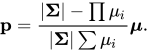
If we let the mean vector of the negative multinomial be $${\displaystyle {\boldsymbol {\mu }}={\frac {x_{0}}{p_{0}}}\mathbf {p} }$$ and covariance matrix $${\displaystyle {\boldsymbol {\Sigma }}={\tfrac {x_{0}}{p_{0}^{2}}}\,\mathbf {p} \mathbf {p} '+{\tfrac {x_{0}}{p_{0}}}\,\operatorname {diag} (\mathbf {p} ),}$$ then it is easy to show through properties of determinants that ${\textstyle |{\boldsymbol {\Sigma }}|={\frac {1}{p_{0}}}\prod _{i=1}^{m}{\mu _{i}}}$. From this, it can be shown that $${\displaystyle x_{0}={\frac {\sum {\mu _{i}}\prod {\mu _{i}}}{|{\boldsymbol {\Sigma }}|-\prod {\mu _{i}}}}}$$ and $${\displaystyle \mathbf {p} ={\frac {|{\boldsymbol {\Sigma }}|-\prod {\mu _{i}}}{|{\boldsymbol {\Sigma }}|\sum {\mu _{i}}}}{\boldsymbol {\mu }}.}$$

Substituting sample moments yields the method of moments estimates $${\displaystyle {\hat {x}}_{0}={\frac {(\sum _{i=1}^{m}{{\bar {x_{i}}})}\prod _{i=1}^{m}{\bar {x_{i}}}}{|\mathbf {S} |-\prod _{i=1}^{m}{\bar {x_{i}}}}}}$$ and $${\displaystyle {\hat {\mathbf {p} }}=\left({\frac {|{\boldsymbol {S}}|-\prod _{i=1}^{m}{{\bar {x}}_{i}}}{|{\boldsymbol {S}}|\sum _{i=1}^{m}{{\bar {x}}_{i}}}}\right){\boldsymbol {\bar {x}}}}$$

• Negative binomial distribution
• Multinomial distribution
• Inverted Dirichlet distribution, a conjugate prior for the negative multinomial
• Dirichlet negative multinomial distribution

Waller LA and Zelterman D. (1997). Log-linear modeling with the negative multi- nomial distribution. Biometrics 53: 971–82.

Johnson, Norman L.; Kotz, Samuel; Balakrishnan, N. (1997). "Chapter 36: Negative Multinomial and Other Multinomial-Related Distributions". Discrete Multivariate Distributions. Wiley. ISBN 978-0-471-12844-1.