Explore Black History

Nonlinear mixed-effects models constitute a class of statistical models generalizing linear mixed-effects models. Like linear mixed-effects models, they are particularly useful in settings where there are multiple measurements within the same statistical units or when there are dependencies between measurements on related statistical units. Nonlinear mixed-effects models are applied in many fields including medicine, public health, pharmacology, and ecology.^[1][2]

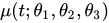
While any statistical model containing both fixed effects and random effects is an example of a nonlinear mixed-effects model, the most commonly used models are members of the class of nonlinear mixed-effects models for repeated measures^[1]

${\displaystyle {y}_{ij}=f(\phi _{ij},{v}_{ij})+\epsilon _{ij},\quad i=1,\ldots ,M,\,j=1,\ldots ,n_{i}}$

where

• ${\displaystyle M}$ is the number of groups/subjects,
• ${\displaystyle n_{i}}$ is the number of observations for the ${\displaystyle i}$th group/subject,
• ${\displaystyle f}$ is a real-valued differentiable function of a group-specific parameter vector ${\displaystyle \phi _{ij}}$ and a covariate vector ${\displaystyle v_{ij}}$,
• ${\displaystyle \phi _{ij}}$ is modeled as a linear mixed-effects model ${\displaystyle \phi _{ij}={\boldsymbol {A}}_{ij}\beta +{\boldsymbol {B}}_{ij}{\boldsymbol {b}}_{i},}$ where ${\displaystyle \beta }$ is a vector of fixed effects and ${\displaystyle {\boldsymbol {b}}_{i}}$ is a vector of random effects associated with group ${\displaystyle i}$, and
• ${\displaystyle \epsilon _{ij}}$ is a random variable describing additive noise.

When the model is only nonlinear in fixed effects and the random effects are Gaussian, maximum-likelihood estimation can be done using nonlinear least squares methods, although asymptotic properties of estimators and test statistics may differ from the conventional general linear model. In the more general setting, there exist several methods for doing maximum-likelihood estimation or maximum a posteriori estimation in certain classes of nonlinear mixed-effects models – typically under the assumption of normally distributed random variables. A popular approach is the Lindstrom-Bates algorithm^[3] which relies on iteratively optimizing a nonlinear problem, locally linearizing the model around this optimum and then employing conventional methods from linear mixed-effects models to do maximum likelihood estimation. Stochastic approximation of the expectation-maximization algorithm gives an alternative approach for doing maximum-likelihood estimation.^[4]

Nonlinear mixed-effects models have been used for modeling progression of disease.^[5] In progressive disease, the temporal patterns of progression on outcome variables may follow a nonlinear temporal shape that is similar between patients. However, the stage of disease of an individual may not be known or only partially known from what can be measured. Therefore, a latent time variable that describe individual disease stage (i.e. where the patient is along the nonlinear mean curve) can be included in the model.

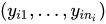
Alzheimer's disease is characterized by a progressive cognitive deterioration. However, patients may differ widely in cognitive ability and reserve, so cognitive testing at a single time point can often only be used to coarsely group individuals in different stages of disease. Now suppose we have a set of longitudinal cognitive data ${\displaystyle (y_{i1},\ldots ,y_{in_{i}})}$ from ${\displaystyle i=1,\ldots ,M}$ individuals that are each categorized as having either normal cognition (CN), mild cognitive impairment (MCI) or dementia (DEM) at the baseline visit (time ${\displaystyle t_{i1}=0}$ corresponding to measurement ${\displaystyle y_{i1}}$). These longitudinal trajectories can be modeled using a nonlinear mixed effects model that allows differences in disease state based on baseline categorization:

${\displaystyle {y}_{ij}=f_{\tilde {\beta }}(t_{ij}+A_{i}^{MCI}\beta ^{MCI}+A_{i}^{DEM}\beta ^{DEM}+b_{i})+\epsilon _{ij},\quad i=1,\ldots ,M,\,j=1,\ldots ,n_{i}}$

where

• ${\displaystyle f_{\tilde {\beta }}}$ is a function that models the mean time-profile of cognitive decline whose shape is determined by the parameters ${\displaystyle {\tilde {\beta }}}$,
• ${\displaystyle t_{ij}}$ represents observation time (e.g. time since baseline in the study),
• ${\displaystyle A_{i}^{MCI}}$ and ${\displaystyle A_{i}^{DEM}}$ are dummy variables that are 1 if individual ${\displaystyle i}$ has MCI or dementia at baseline and 0 otherwise,
• ${\displaystyle \beta ^{MCI}}$ and ${\displaystyle \beta ^{DEM}}$ are parameters that model the difference in disease progression of the MCI and dementia groups relative to the cognitively normal,
• ${\displaystyle b_{i}}$ is the difference in disease stage of individual ${\displaystyle i}$ relative to his/her baseline category, and
• ${\displaystyle \epsilon _{ij}}$ is a random variable describing additive noise.

An example of such a model with an exponential mean function fitted to longitudinal measurements of the Alzheimer's Disease Assessment Scale-Cognitive Subscale (ADAS-Cog) is shown in the box. As shown, the inclusion of fixed effects of baseline categorization (MCI or dementia relative to normal cognition) and the random effect of individual continuous disease stage ${\displaystyle b_{i}}$ aligns the trajectories of cognitive deterioration to reveal a common pattern of cognitive decline.

Growth phenomena often follow nonlinear patters (e.g. logistic growth, exponential growth, and hyperbolic growth). Factors such as nutrient deficiency may both directly affect the measured outcome (e.g. organisms with lack of nutrients end up smaller), but possibly also timing (e.g. organisms with lack of nutrients grow at a slower pace). If a model fails to account for the differences in timing, the estimated population-level curves may smooth out finer details due to lack of synchronization between organisms. Nonlinear mixed-effects models enable simultaneous modeling of individual differences in growth outcomes and timing.

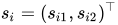
Models for estimating the mean curves of human height and weight as a function of age and the natural variation around the mean are used to create growth charts. The growth of children can however become desynchronized due to both genetic and environmental factors. For example, age at onset of puberty and its associated height spurt can vary several years between adolescents. Therefore, cross-sectional studies may underestimate the magnitude of the pubertal height spurt because age is not synchronized with biological development. The differences in biological development can be modeled using random effects ${\displaystyle {\boldsymbol {w}}_{i}}$ that describe a mapping of observed age to a latent biological age using a so-called warping function ${\displaystyle v(\cdot ,{\boldsymbol {w}}_{i})}$. A simple nonlinear mixed-effects model with this structure is given by

${\displaystyle {y}_{ij}=f_{\beta }(v(t_{ij},{\boldsymbol {w}}_{i}))+\epsilon _{ij},\quad i=1,\ldots ,M,\,j=1,\ldots ,n_{i}}$

where

• ${\displaystyle f_{\beta }}$ is a function that represents the height development of a typical child as a function of age. Its shape is determined by the parameters ${\displaystyle \beta }$,
• ${\displaystyle t_{ij}}$ is the age of child ${\displaystyle i}$ corresponding to the height measurement ${\displaystyle y_{ij}}$,
• ${\displaystyle v(\cdot ,{\boldsymbol {w}}_{i})}$ is a warping function that maps age to biological development to synchronize. Its shape is determined by the random effects ${\displaystyle {\boldsymbol {w}}_{i}}$,
• ${\displaystyle \epsilon _{ij}}$ is a random variable describing additive variation (e.g. consistent differences in height between children and measurement noise).

There exists several methods and software packages for fitting such models. The so-called SITAR model^[7] can fit such models using warping functions that are affine transformations of time (i.e. additive shifts in biological age and differences in rate of maturation). SITAR can be employed as a sophisticated data reduction tool, reducing growth trajectories to three patient level effects summarising the variability in 'size', 'timing' and 'intensity' of growth across a sample. This can facilitate the assessment of the impact of predictor variables on overall growth trajectory, and has been used to quantify the impact of antenatal steroids on child growth.^[8] An alternative approach is the so-called pavpop model^[6] that can fit models with smoothly-varying warping functions, an example of which is shown in the box.

PK/PD models for describing exposure-response relationships such as the Emax model can be formulated as nonlinear mixed-effects models.^[9] The mixed-model approach allows modeling of both population level and individual differences in effects that have a nonlinear effect on the observed outcomes, for example the rate at which a compound is being metabolized or distributed in the body.

The platform of the nonlinear mixed effect models can be used to describe infection trajectories of subjects and understand some common features shared across the subjects. In epidemiological problems, subjects can be countries, states, or counties, etc. This can be particularly useful in estimating a future trend of the epidemic in an early stage of pendemic where nearly little information is known regarding the disease.^[10]

The eventual success of petroleum development projects relies on a large degree of well construction costs. As for unconventional oil and gas reservoirs, because of very low permeability, and a flow mechanism very different from that of conventional reservoirs, estimates for the well construction cost often contain high levels of uncertainty, and oil companies need to make heavy investment in the drilling and completion phase of the wells. The overall recent commercial success rate of horizontal wells in the United States is known to be 65%, which implies that only 2 out of 3 drilled wells will be commercially successful. For this reason, one of the crucial tasks of petroleum engineers is to quantify the uncertainty associated with oil or gas production from shale reservoirs, and further, to predict an approximated production behavior of a new well at a new location given specific completion data before actual drilling takes place to save a large degree of well construction costs.

The platform of the nonlinear mixed effect models can be extended to consider the spatial association by incorporating the geostatistical processes such as Gaussian process on the second stage of the model as follows:^[11]

${\displaystyle {y}_{it}=\mu (t;\theta _{1i},\theta _{2i},\theta _{3i})+\epsilon _{it},\quad \quad \quad \quad \quad \quad \quad \quad \quad \quad \quad \quad \quad i=1,\ldots ,N,\,t=1,\ldots ,T_{i},}$

${\displaystyle \theta _{li}=\theta _{l}(s_{i})=\alpha _{l}+\sum _{j=1}^{p}\beta _{lj}x_{j}+\epsilon _{l}(s_{i})+\eta _{l}(s_{i}),\quad \epsilon _{l}(\cdot )\sim GWN(\sigma _{l}^{2}),\quad \quad l=1,2,3,}$ ${\displaystyle \eta _{l}(\cdot )\sim GP(0,K_{\gamma _{l}}(\cdot ,\cdot )),\quad K_{\gamma _{l}}(s_{i},s_{j})=\gamma _{l}^{2}\exp(-e^{\rho _{l}}\|s_{i}-s_{j}\|^{2}),\quad \quad \quad l=1,2,3,}$ ${\displaystyle \beta _{lj}|\lambda _{lj},\tau _{l},\sigma _{l}\sim N(0,\sigma _{l}^{2}\tau _{l}^{2}\lambda _{lj}^{2}),\quad \sigma ,\lambda _{lj},\tau _{l},\sigma _{l}\sim C^{+}(0,1),\quad \quad \quad \quad \quad \quad \quad l=1,2,3,\,j=1,\cdots ,p,}$ ${\displaystyle \alpha _{l}\sim \pi (\alpha )\propto 1,\quad \sigma _{l}^{2}\sim \pi (\sigma ^{2})\propto 1/\sigma ^{2},\quad \quad \quad \quad \quad \quad \quad \quad \quad \quad \quad \quad \quad l=1,2,3,}$

where

• ${\displaystyle \mu (t;\theta _{1},\theta _{2},\theta _{3})}$ is a function that models the mean time-profile of log-scaled oil production rate whose shape is determined by the parameters ${\displaystyle (\theta _{1},\theta _{2},\theta _{3})}$. The function is obtained from taking logarithm to the rate decline curve used in decline curve analysis,
• ${\displaystyle x_{i}=(x_{i1},\cdots ,x_{ip})^{\top }}$ represents covariates obtained from the completion process of the hydraulic fracturing and horizontal directional drilling for the ${\displaystyle i}$-th well,
• ${\displaystyle s_{i}=(s_{i1},s_{i2})^{\top }}$ represents the spatial location (longitude, latitude) of the ${\displaystyle i}$-th well,
• ${\displaystyle \epsilon _{l}(\cdot )}$ represents the Gaussian white noise with error variance ${\displaystyle \sigma _{l}^{2}}$ (also called the nugget effect),
• ${\displaystyle \eta _{l}(\cdot )}$ represents the Gaussian process with Gaussian covariance function ${\displaystyle K_{\gamma _{l}}(\cdot ,\cdot )}$,
• ${\displaystyle \beta }$ represents the horseshoe shrinkage prior.

The Gaussian process regressions used on the latent level (the second stage) eventually produce kriging predictors for the curve parameters ${\displaystyle (\theta _{1i},\theta _{2i},\theta _{3i}),(i=1,\cdots ,N),}$ that dictate the shape of the mean curve ${\displaystyle \mu (t;\theta _{1},\theta _{2},\theta _{3})}$ on the date level (the first level). As the kriging techniques have been employed in the latent level, this technique is called latent kriging. The right panels show the prediction results of the latent kriging method applied to the two test wells in the Eagle Ford Shale Reservoir of South Texas.

The framework of Bayesian hierarchical modeling is frequently used in diverse applications. Particularly, Bayesian nonlinear mixed-effects models have recently received significant attention. A basic version of the Bayesian nonlinear mixed-effects models is represented as the following three-stage:

Stage 1: Individual-Level Model

${\displaystyle {y}_{ij}=f(t_{ij};\theta _{1i},\theta _{2i},\ldots ,\theta _{li},\ldots ,\theta _{Ki})+\epsilon _{ij},\quad \epsilon _{ij}\sim N(0,\sigma ^{2}),\quad i=1,\ldots ,N,\,j=1,\ldots ,M_{i}.}$

Stage 2: Population Model

${\displaystyle \theta _{li}=\alpha _{l}+\sum _{b=1}^{P}\beta _{lb}x_{ib}+\eta _{li},\quad \eta _{li}\sim N(0,\omega _{l}^{2}),\quad i=1,\ldots ,N,\,l=1,\ldots ,K.}$

Stage 3: Prior

${\displaystyle \sigma ^{2}\sim \pi (\sigma ^{2}),\quad \alpha _{l}\sim \pi (\alpha _{l}),\quad (\beta _{l1},\ldots ,\beta _{lb},\ldots ,\beta _{lP})\sim \pi (\beta _{l1},\ldots ,\beta _{lb},\ldots ,\beta _{lP}),\quad \omega _{l}^{2}\sim \pi (\omega _{l}^{2}),\quad l=1,\ldots ,K.}$

Here, ${\displaystyle y_{ij}}$ denotes the continuous response of the ${\displaystyle i}$-th subject at the time point ${\displaystyle t_{ij}}$, and ${\displaystyle x_{ib}}$ is the ${\displaystyle b}$-th covariate of the ${\displaystyle i}$-th subject. Parameters involved in the model are written in Greek letters. ${\displaystyle f(t;\theta _{1},\ldots ,\theta _{K})}$ is a known function parameterized by the ${\displaystyle K}$-dimensional vector ${\displaystyle (\theta _{1},\ldots ,\theta _{K})}$. Typically, ${\displaystyle f}$ is a `nonlinear' function and describes the temporal trajectory of individuals. In the model, ${\displaystyle \epsilon _{ij}}$ and ${\displaystyle \eta _{li}}$ describe within-individual variability and between-individual variability, respectively. If Stage 3: Prior is not considered, then the model reduces to a frequentist nonlinear mixed-effect model.

A central task in the application of the Bayesian nonlinear mixed-effect models is to evaluate the posterior density:

${\displaystyle \pi (\{\theta _{li}\}_{i=1,l=1}^{N,K},\sigma ^{2},\{\alpha _{l}\}_{l=1}^{K},\{\beta _{lb}\}_{l=1,b=1}^{K,P},\{\omega _{l}\}_{l=1}^{K}|\{y_{ij}\}_{i=1,j=1}^{N,M_{i}})}$

${\displaystyle \propto \pi (\{y_{ij}\}_{i=1,j=1}^{N,M_{i}},\{\theta _{li}\}_{i=1,l=1}^{N,K},\sigma ^{2},\{\alpha _{l}\}_{l=1}^{K},\{\beta _{lb}\}_{l=1,b=1}^{K,P},\{\omega _{l}\}_{l=1}^{K})}$

${\displaystyle =\underbrace {\pi (\{y_{ij}\}_{i=1,j=1}^{N,M_{i}}|\{\theta _{li}\}_{i=1,l=1}^{N,K},\sigma ^{2})} _{Stage1:Individual-LevelModel}\times \underbrace {\pi (\{\theta _{li}\}_{i=1,l=1}^{N,K}|\{\alpha _{l}\}_{l=1}^{K},\{\beta _{lb}\}_{l=1,b=1}^{K,P},\{\omega _{l}\}_{l=1}^{K})} _{Stage2:PopulationModel}\times \underbrace {p(\sigma ^{2},\{\alpha _{l}\}_{l=1}^{K},\{\beta _{lb}\}_{l=1,b=1}^{K,P},\{\omega _{l}\}_{l=1}^{K})} _{Stage3:Prior}}$

The panel on the right displays Bayesian research cycle using Bayesian nonlinear mixed-effects model.^[13] A research cycle using the Bayesian nonlinear mixed-effects model comprises two steps: (a) standard research cycle and (b) Bayesian-specific workflow. Standard research cycle involves literature review, defining a problem and specifying the research question and hypothesis. Bayesian-specific workflow comprises three sub-steps: (b)–(i) formalizing prior distributions based on background knowledge and prior elicitation; (b)–(ii) determining the likelihood function based on a nonlinear function ${\displaystyle f}$; and (b)–(iii) making a posterior inference. The resulting posterior inference can be used to start a new research cycle.

• Mixed model
• Fixed effects model
• Generalized linear mixed model
• Linear regression
• Mixed-design analysis of variance
• Multilevel model
• Random effects model
• Repeated measures design

• Hajjem, Ahlem; Bellavance, François; Larocque, Denis (2011). "Mixed effects regression trees for clustered data". Statistics & Probability Letters. 81 (4): 451–459. doi:10.1016/j.spl.2010.12.003. ISSN 0167-7152.
• Hajjem, Ahlem; Larocque, Denis; Bellavance, François (2017). "Generalized mixed effects regression trees". Statistics & Probability Letters. 126: 114–118. doi:10.1016/j.spl.2017.02.033. ISSN 0167-7152.
• Hajjem, Ahlem; Bellavance, François; Larocque, Denis (2014-06-03). "Mixed-effects random forest for clustered data". Journal of Statistical Computation and Simulation. 84 (6): 1313–1328. doi:10.1080/00949655.2012.741599. ISSN 0094-9655.