Explore Black History

This article needs more citations. Please help improve this article by adding citations to reliable sources. Unsourced material may be challenged and removed. Find sources: "Root locus analysis" – news · newspapers · books · scholar · JSTOR (January 2008) (Learn how and when to remove this message)

This article includes a list of general references but lacks sufficient corresponding inline citations. Please help improve this article by introducing more precise citations. (December 2022) (Learn how and when to remove this message)

In control theory and stability theory, root locus analysis is a graphical method for examining how the roots of a linear time-invariant (LTI) system change with variation of a certain system parameter, commonly a gain within a feedback system. This is a technique used as a stability criterion in the field of classical control theory developed by Walter R. Evans which can determine stability of the system. The root locus plots the poles of the closed loop transfer function in the complex s-plane as a function of a gain parameter (see pole–zero plot).

Evans also invented in 1948 an analog computer to compute root loci, called a "Spirule" (after "spiral" and "slide rule"); it found wide use before the advent of digital computers.^{[1][2][3][4][5][6][7][8][9]}

If a pole sits at a location ${\displaystyle s=\sigma +j\omega }$, then the system contains a mode ${\displaystyle y_{mode}(t)\propto e^{\sigma t}\cos {(\omega t+\phi )}}$ with growth rate σ and phase offset φ at the oscillation frequency ω. All modes must have negative growth rates for the system to be asymptotically stable. This stability condition is often phrased as all poles needing to lie in the left hand plane, i.e. ${\displaystyle \sigma <0}$. For stable modes, the (positive) decay rate is then -σ. When single complex pairs of poles lie on the imaginary axis ${\displaystyle \sigma =0}$ (excluding the origin), the system is considered to be marginally stable.

In addition to determining the stability of the system, the root locus can be used to design the damping ratio (ζ) and natural frequency (ω_n) of a feedback system. Lines of constant damping ratio can be drawn radially from the origin (with angle ${\displaystyle \cos ^{-1}(\zeta )}$ from the negative real axis), and lines of constant natural frequency can be drawn as circles centered at the origin with radius ω_n. By selecting a point along the root locus that coincides with a desired damping ratio and natural frequency, a gain K can be calculated and implemented in the controller. More elaborate techniques of controller design using the root locus are available in most control textbooks: for instance, lead, lag, PI, PD and PID controllers can be designed approximately with this technique.

The definition of the damping ratio and natural frequency in the paragraph above presumes that the overall feedback system is stable and well approximated by a second-order system. This happens when the system satisfies the "dominant poles" approximation. A complex pair of poles dominates when every other pole lies sufficiently farther left, e.g. ${\displaystyle |\sigma |>5|\sigma _{dom}|}$. Equivalently, the dominant poles are the one with the smallest decay rate ${\displaystyle -\sigma _{dom}}$. A single pole on the real axis might also dominate, in which case the system can be approximated as a first-order system. Note that the factor of 5 is a common heuristic rather than a rule, derived from ${\displaystyle e^{-5}<1\%}$. Additionally, nearby zeros may weaken the effect of poles. So all controllers designed with this approximation should be simulated with the full transfer function to verify that the design goals are satisfied.

The root locus of a LTI feedback system is the graphical representation in the complex s-plane of the possible locations of its closed-loop poles for varying values of a certain system parameter. The points that are part of the root locus satisfy the angle condition. The value of the parameter for a certain point of the root locus can be obtained using the magnitude condition.

Suppose there is a LTI feedback system with input signal ${\displaystyle X(s)}$ and output signal ${\displaystyle Y(s)}$. The forward path transfer function is ${\displaystyle G(s)}$; the feedback path transfer function is ${\displaystyle H(s)}$.

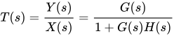
For this system, the closed-loop transfer function is given by^[10]

${\displaystyle T(s)={\frac {Y(s)}{X(s)}}={\frac {G(s)}{1+G(s)H(s)}}}$

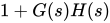
Thus, the closed-loop poles of the closed-loop transfer function are the roots of the characteristic polynomial ${\displaystyle 1+G(s)H(s)}$. The roots of this polynomial may be found wherever the equation ${\displaystyle 1+G(s)H(s)=0}$ holds.

In systems without pure delay, the product ${\displaystyle G(s)H(s)}$ is a rational polynomial function and may be expressed as^[11]

${\displaystyle G(s)H(s)=K{\frac {(s+z_{1})(s+z_{2})\cdots (s+z_{m})}{(s+p_{1})(s+p_{2})\cdots (s+p_{n})}}}$

where ${\displaystyle -z_{i}}$ are the ${\displaystyle m}$ zeros, ${\displaystyle -p_{i}}$ are the ${\displaystyle n}$ poles, and ${\displaystyle K}$ is a scalar gain. Typically, a root locus diagram will indicate the transfer function's pole locations for varying values of the parameter ${\displaystyle K}$. A root locus plot will be all those points in the s-plane where ${\displaystyle G(s)H(s)=-1}$ for any value of ${\displaystyle K}$.

The factoring of ${\displaystyle K}$ and the use of simple monomials means the evaluation of the rational polynomial can be done with vector techniques that add or subtract angles and multiply or divide magnitudes. The vector formulation arises from the fact that each monomial term ${\displaystyle (s-a)}$ in the factored ${\displaystyle G(s)H(s)}$ represents the vector from ${\displaystyle a}$ to ${\displaystyle s}$ in the s-plane. The polynomial can be evaluated by considering the magnitudes and angles of each of these vectors.

According to vector mathematics, the angle of the result of the rational polynomial is the sum of all the angles in the numerator minus the sum of all the angles in the denominator. So to test whether a point in the s-plane is on the root locus, only the angles to all the open loop poles and zeros need be considered. This is known as the angle condition.

Similarly, the magnitude of the result of the rational polynomial is the product of all the magnitudes in the numerator divided by the product of all the magnitudes in the denominator. It turns out that the calculation of the magnitude is not needed to determine if a point in the s-plane is part of the root locus because ${\displaystyle K}$ varies and can take an arbitrary real value. For each point of the root locus a value of ${\displaystyle K}$ can be calculated. This is known as the magnitude condition.

The root locus only gives the location of closed loop poles as the gain ${\displaystyle K}$ is varied. The value of ${\displaystyle K}$ does not affect the location of the zeros. The open-loop zeros are the same as the closed-loop zeros.

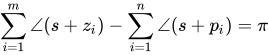
A point ${\displaystyle s}$ of the complex s-plane satisfies the angle condition if

${\displaystyle \angle (G(s)H(s))=\pi }$

which is the same as saying that

${\displaystyle \sum _{i=1}^{m}\angle (s+z_{i})-\sum _{i=1}^{n}\angle (s+p_{i})=\pi }$

that is, the sum of the angles from the open-loop zeros to the point ${\displaystyle s}$ (measured per zero w.r.t. a horizontal running through that zero) minus the angles from the open-loop poles to the point ${\displaystyle s}$ (measured per pole w.r.t. a horizontal running through that pole) has to be equal to ${\displaystyle \pi }$, or 180 degrees. Note that these interpretations should not be mistaken for the angle differences between the point ${\displaystyle s}$ and the zeros/poles.

A value of ${\displaystyle K}$ satisfies the magnitude condition for a given ${\displaystyle s}$ point of the root locus if

${\displaystyle |G(s)H(s)|=1}$

which is the same as saying that

${\displaystyle K{\frac {|s+z_{1}||s+z_{2}|\cdots |s+z_{m}|}{|s+p_{1}||s+p_{2}|\cdots |s+p_{n}|}}=1}$.

Using a few basic rules, the root locus method can plot the overall shape of the path (locus) traversed by the roots as the value of ${\displaystyle K}$ varies. The plot of the root locus then gives an idea of the stability and dynamics of this feedback system for different values of ${\displaystyle K}$.^[12][13] The rules are the following:

• Mark open-loop poles and zeros
• Mark real axis portion to the left of an odd number of poles and zeros
• Find asymptotes

Let P be the number of poles and Z be the number of zeros:

${\displaystyle P-Z={\text{number of asymptotes}}\,}$

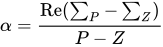
The asymptotes intersect the real axis at ${\displaystyle \alpha }$ (which is called the centroid) and depart at angle ${\displaystyle \phi }$ given by:

${\displaystyle \phi _{l}={\frac {180^{\circ }+(l-1)360^{\circ }}{P-Z}},l=1,2,\ldots ,P-Z}$

${\displaystyle \alpha ={\frac {\operatorname {Re} \left(\sum _{P}-\sum _{Z}\right)}{P-Z}}}$

where ${\displaystyle \sum _{P}}$ is the sum of all the locations of the poles, ${\displaystyle \sum _{Z}}$ is the sum of all the locations of the explicit zeros and ${\displaystyle \operatorname {Re} ()}$ denotes that we are only interested in the real part.

• Phase condition on test point to find angle of departure
• Compute breakaway/break-in points

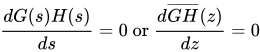
The breakaway points are located at the roots of the following equation:

${\displaystyle {\frac {dG(s)H(s)}{ds}}=0{\text{ or }}{\frac {d{\overline {GH}}(z)}{dz}}=0}$

Once you solve for z, the real roots give you the breakaway/reentry points. Complex roots correspond to a lack of breakaway/reentry.

Given the general closed-loop denominator rational polynomial

${\displaystyle 1+G(s)H(s)=1+K{\frac {b_{m}s^{m}+\ldots +b_{1}s+b_{0}}{s^{n}+a_{n-1}s^{n-1}+\ldots +a_{1}s+a_{0}}},}$

the characteristic equation can be simplified to

${\displaystyle s^{n}+a_{n-1}s^{n-1}+\ldots +(a_{m}+Kb_{m})s^{m}+\ldots +(a_{1}+Kb_{1})s+(a_{0}+Kb_{0})=0.}$

The solutions of ${\displaystyle s}$ to this equation are the root loci of the closed-loop transfer function.

Given

${\displaystyle 1+G(s)H(s)=1+K{\frac {s+3}{s^{3}+3s^{2}+5s+1}},}$

we will have the characteristic equation

${\displaystyle s^{3}+3s^{2}+(5+K)s+(1+3K)=0.}$

The following MATLAB code will plot the root locus of the closed-loop transfer function as ${\displaystyle K}$ varies using the described manual method as well as the rlocus built-in function:

% Manual method
K_array = (0:0.1:220).'; % .' is a transpose. Looking up in Matlab documentation.
NK = length(K_array);
x_array = zeros(NK, 3);
y_array = zeros(NK, 3);

for nK = 1:NK
   K = K_array(nK);
   C = [1, 3, (5 + K), (1 + 3*K)];
   r = roots(C).';
   x_array(nK,:) = real(r);
   y_array(nK,:) = imag(r);
end

figure();
plot(x_array, y_array);
grid on;

% Built-in method
sys = tf([1, 3], [1, 3, 5, 1]);
figure();
rlocus(sys);

The following Python code can also be used to calculate and plot the root locus of the closed-loop transfer function using the Python Control Systems Library^[14] and Matplotlib^[15].

import control as ct
import matplotlib.pyplot as plt

# Define the transfer function
sys = ct.TransferFunction([1, 3], [1, 3, 5, 1])

# Calculate and plot the root locus
roots, gains = ct.root_locus(sys, plot=True)
plt.show()

The root locus method can also be used for the analysis of sampled data systems by computing the root locus in the z-plane, the discrete counterpart of the s-plane. The equation z = e^sT maps continuous s-plane poles (not zeros) into the z-domain, where T is the sampling period. The stable, left half s-plane maps into the interior of the unit circle of the z-plane, with the s-plane origin equating to |z| = 1 (because e⁰ = 1). A diagonal line of constant damping in the s-plane maps around a spiral from (1,0) in the z plane as it curves in toward the origin. The Nyquist aliasing criteria is expressed graphically in the z-plane by the x-axis, where ωnT = π. The line of constant damping just described spirals in indefinitely but in sampled data systems, frequency content is aliased down to lower frequencies by integral multiples of the Nyquist frequency. That is, the sampled response appears as a lower frequency and better damped as well since the root in the z-plane maps equally well to the first loop of a different, better damped spiral curve of constant damping. Many other interesting and relevant mapping properties can be described, not least that z-plane controllers, having the property that they may be directly implemented from the z-plane transfer function (zero/pole ratio of polynomials), can be imagined graphically on a z-plane plot of the open loop transfer function, and immediately analyzed utilizing root locus.

Since root locus is a graphical angle technique, root locus rules work the same in the z and s planes.

The idea of a root locus can be applied to many systems where a single parameter K is varied. For example, it is useful to sweep any system parameter for which the exact value is uncertain in order to determine its behavior.

• Phase margin
• Routh–Hurwitz stability criterion
• Nyquist stability criterion
• Gain and phase margin
• Bode plot

• Kuo, Benjamin C. (1967). "Root Locus Technique". Automatic Control Systems (second ed.). Englewood Cliffs, NJ: Prentice-Hall. pp. 329–388. ASIN B000KPT04C. LCCN 67016388. OCLC 3805225.

• Ash, R. H.; Ash, G. H. (October 1968), "Numerical Computation of Root Loci Using the Newton-Raphson Technique", IEEE Transactions on Automatic Control, 13 (5): 576–582, doi:10.1109/TAC.1968.1098980
• Williamson, S. E. (May 1968), "Design Data to assist the Plotting of Root Loci (Part I)", Control Magazine, 12 (119): 404–407
• Williamson, S. E. (June 1968), "Design Data to assist the Plotting of Root Loci (Part II)", Control Magazine, 12 (120): 556–559
• Williamson, S. E. (July 1968), "Design Data to assist the Plotting of Root Loci (Part III)", Control Magazine, 12 (121): 645–647
• Williamson, S. E. (May 15, 1969), "Computer Program to Obtain the Time Response of Sampled Data Systems", Electronics Letters, 5 (10): 209–210, Bibcode:1969ElL.....5..209W, doi:10.1049/el:19690159
• Williamson, S. E. (July 1969), "Accurate root locus plotting including the effects of pure time delay. Computer-program description", Proceedings of the Institution of Electrical Engineers, 116 (7): 1269–1271, doi:10.1049/piee.1969.0235, archived from the original on June 29, 2019

• Wikibooks: Control Systems/Root Locus
• Carnegie Mellon / University of Michigan Tutorial
• Excellent examples. Start with example 5 and proceed backwards through 4 to 1. Also visit the main page
• The root-locus method: Drawing by hand techniques
• "RootLocs": A free multi-featured root-locus plotter for Mac and Windows platforms
• "Root Locus": A free root-locus plotter/analyzer for Windows
• Root Locus at ControlTheoryPro.com
• Root Locus Analysis of Control Systems
• MATLAB function for computing root locus of a SISO open-loop model
• Wechsler, E. R. (January–March 1983), "Root Locus Algorithms for Programmable Pocket Calculators" (PDF), Telecommunications and Data Acquisition Progress Report, 73, NASA: 60–64, Bibcode:1983TDAPR..73...60W
• Mathematica function for plotting the root locus