Explore Black History

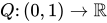
In probability and statistics, the quantile function of a probability distribution is the inverse of its cumulative distribution function. That is, the quantile function of a distribution ${\displaystyle {\mathcal {D}}}$ is the function ${\displaystyle Q}$ such that ${\displaystyle \Pr \left[\mathrm {X} \leq Q(p)\right]=p}$ for any random variable ${\displaystyle \mathrm {X} \sim {\mathcal {D}}}$ and probability ${\displaystyle p\in (0,1)}$.

The quantile function is also called the percentile function (after the percentile), percent-point function, inverse cumulative distribution function or inverse distribution function.

With reference to a continuous and strictly increasing cumulative distribution function (c.d.f.) ${\displaystyle F_{X}\colon \mathbb {R} \to [0,1]}$ of a random variable X, the quantile function ${\displaystyle Q\colon (0,1)\to \mathbb {R} }$ maps its input p to a threshold value x so that the probability of X being less or equal than x is p. In terms of the distribution function F, the quantile function Q returns the value x such that

$${\displaystyle F_{X}(x):=\Pr(X\leq x)=p,}$$

which can be written as the inverse function of the cumulative distribution function.

$${\displaystyle Q(p)=F_{X}^{-1}(p).}$$

In the general case of distribution functions that lack strict monotonicity or continuity, and therefore do not permit an inverse c.d.f., the quantile is a (potentially) set valued functional of a distribution function F, given by the interval

$${\displaystyle {\begin{aligned}Q(p)&={\big [}\sup\{x\colon F(x)<p\},\ \sup\{x\colon F(x)\leq p\}{\big ]}\\&={\big [}\inf\{x\colon F(x)\geq p\},\ \inf\{x\colon F(x)>p\}{\big ]}.\end{aligned}}}$$

The first interval^[1] is equivalent to the second interval because of the (non-strict) monotonicity of F.^{[Note 1]}

It is often standard to choose the lowest value, which can equivalently be written as

$${\displaystyle Q(p)=\inf\{x\in \mathbb {R} :p\leq F(x)\}.}$$

Here we capture the fact that the quantile function returns the minimum value of x from amongst all those values whose c.d.f value exceeds p, which is equivalent to the previous probability statement in the special case that the distribution is continuous.

The quantile is also the unique function satisfying the Galois inequalities

$${\displaystyle Q(p)\leq x}$$ if and only if ${\displaystyle p\leq F(x).}$

If the function F is continuous and strictly monotonically increasing, then the inequalities can be replaced by equalities, and we have

$${\displaystyle Q=F^{-1}.}$$

In general, even though the distribution function F may fail to possess a left or right inverse, the quantile function Q behaves as an "almost sure left inverse" for the distribution function, in the sense that

$${\displaystyle Q{\bigl (}F(X){\bigr )}=X\quad {\text{almost surely.}}}$$

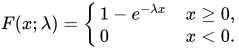
For example, the cumulative distribution function of Exponential(λ) (i.e. intensity λ and expected value (mean) 1/λ) is

$${\displaystyle F(x;\lambda )={\begin{cases}1-e^{-\lambda x}&x\geq 0,\\0&x<0.\end{cases}}}$$

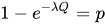
The quantile function for Exponential(λ) is derived by finding the value of Q for which ${\displaystyle 1-e^{-\lambda Q}=p}$:

$${\displaystyle Q(p;\lambda )={\frac {-\ln(1-p)}{\lambda }},}$$

for 0 ≤ p < 1. The quartiles are therefore:

first quartile (p = 1/4)

${\displaystyle -\ln(3/4)/\lambda ,}$

median (p = 2/4)

${\displaystyle -\ln(1/2)/\lambda ,}$

third quartile (p = 3/4)

${\displaystyle -\ln(1/4)/\lambda .}$

Quantile functions are used in both statistical applications and Monte Carlo methods.

The quantile function is one way of prescribing a probability distribution, and it is an alternative to the probability density function (pdf) or probability mass function, the cumulative distribution function (cdf) and the characteristic function. The quantile function, Q, of a probability distribution is the inverse of its cumulative distribution function F. The derivative of the quantile function, namely the quantile density function, is yet another way of prescribing a probability distribution. It is the reciprocal of the pdf composed with the quantile function.

Consider a statistical application where a user needs to know key percentage points of a given distribution. For example, they require the median and 25% and 75% quartiles as in the example above or 5%, 95%, 2.5%, 97.5% levels for other applications such as assessing the statistical significance of an observation whose distribution is known; see the quantile entry. Before the popularization of computers, it was not uncommon for books to have appendices with statistical tables sampling the quantile function.^[2] Statistical applications of quantile functions are discussed extensively by Gilchrist.^[3]

Monte-Carlo simulations employ quantile functions to produce non-uniform random or pseudorandom numbers for use in diverse types of simulation calculations. A sample from a given distribution may be obtained in principle by applying its quantile function to a sample from a uniform distribution. The demands of simulation methods, for example in modern computational finance, are focusing increasing attention on methods based on quantile functions, as they work well with multivariate techniques based on either copula or quasi-Monte-Carlo methods^[4] and Monte Carlo methods in finance.

The integral of the quantile function is used to compute the Lorenz curve in economics and conditional value at risk in finance.

The evaluation of quantile functions often involves numerical methods, such as the exponential distribution above, which is one of the few distributions where a closed-form expression can be found (others include the uniform, the Weibull, the Tukey lambda (which includes the logistic) and the log-logistic). When the cdf itself has a closed-form expression, one can always use a numerical root-finding algorithm such as the bisection method to invert the cdf. Other methods rely on an approximation of the inverse via interpolation techniques.^[5][6] Further algorithms to evaluate quantile functions are given in the Numerical Recipes series of books. Algorithms for common distributions are built into many statistical software packages. General methods to numerically compute the quantile functions for general classes of distributions can be found in the following libraries:

• C library UNU.RAN ^[7]
• R library Runuran ^[8]
• Python subpackage sampling in scipy.stats^[9][10]

Quantile functions may also be characterized as solutions of non-linear ordinary and partial differential equations. The ordinary differential equations for the cases of the normal, Student, beta and gamma distributions have been given and solved.^[11]

The normal distribution is perhaps the most important case. Because the normal distribution is a location-scale family, its quantile function for arbitrary parameters can be derived from a simple transformation of the quantile function of the standard normal distribution, known as the probit function. Unfortunately, this function has no closed-form representation using basic algebraic functions; as a result, approximate representations are usually used. Thorough composite rational and polynomial approximations have been given by Wichura^[12] and Acklam.^[13] Non-composite rational approximations have been developed by Shaw.^[14]

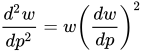
A non-linear ordinary differential equation for the normal quantile, w(p), may be given. It is

$${\displaystyle {\frac {d^{2}w}{dp^{2}}}=w\left({\frac {dw}{dp}}\right)^{2}}$$

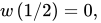
with the centre (initial) conditions

$${\displaystyle w\left(1/2\right)=0,\,}$$ $${\displaystyle w'\left(1/2\right)={\sqrt {2\pi }}.\,}$$

This equation may be solved by several methods, including the classical power series approach. From this solutions of arbitrarily high accuracy may be developed (see Steinbrecher and Shaw, 2008).

This has historically been one of the more intractable cases, as the presence of a parameter, ν, the degrees of freedom, makes the use of rational and other approximations awkward. Simple formulas exist when the ν = 1, 2, 4 and the problem may be reduced to the solution of a polynomial when ν is even. In other cases the quantile functions may be developed as power series.^[15] The simple cases are as follows:

• ν = 1 (Cauchy distribution): $${\displaystyle Q(p)=\tan \left(\pi \left(p-{\tfrac {1}{2}}\right)\right)\,;}$$
• v = 2: $${\displaystyle Q(p)=2\left(p-{\tfrac {1}{2}}\right){\sqrt {\frac {2}{\alpha }}}\,;}$$
• v = 4: $${\displaystyle Q(p)=2\operatorname {sign} \left(p-{\tfrac {1}{2}}\right){\sqrt {q-1}}\,;}$$

where ⁠${\displaystyle \alpha =4p(1-p)}$⁠, ⁠${\displaystyle \textstyle q={\tfrac {1}{\sqrt {\alpha }}}\cos \left({\tfrac {1}{3}}\arccos \left({\sqrt {\alpha }}\right)\right)}$⁠, and $${\displaystyle \operatorname {sign} x={\begin{cases}-1&{\text{if }}x<0;\\{\hphantom {-}}0&{\text{if }}x=0;\\{\hphantom {-}}1&{\text{if }}x>0.\end{cases}}}$$

Analogously to the mixtures of densities, distributions can be defined as quantile mixtures $${\displaystyle Q(p)=\sum _{i=1}^{m}a_{i}Q_{i}(p),}$$ where ${\displaystyle Q_{i}(p)}$, ${\displaystyle i=1,\ldots ,m}$ are quantile functions and ${\displaystyle a_{i}}$, ${\displaystyle i=1,\ldots ,m}$ are the model parameters. The parameters ${\displaystyle a_{i}}$ must be selected so that ${\displaystyle Q(p)}$ is a quantile function. Two four-parametric quantile mixtures, the normal-polynomial quantile mixture and the Cauchy-polynomial quantile mixture, are presented by Karvanen.^[16]

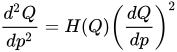
The non-linear ordinary differential equation given for normal distribution is a special case of that available for any quantile function whose second derivative exists. In general the equation for a quantile, Q(p), may be given. It is

$${\displaystyle {\frac {d^{2}Q}{dp^{2}}}=H(Q)\left({\frac {dQ}{dp}}\right)^{2}}$$

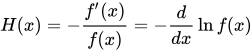
augmented by suitable boundary conditions, where

$${\displaystyle H(x)=-{\frac {f'(x)}{f(x)}}=-{\frac {d}{dx}}\ln f(x)}$$

and f(x) is the probability density function. The forms of this equation, and its classical analysis by series and asymptotic solutions, for the cases of the normal, Student, gamma and beta distributions has been elucidated by Steinbrecher and Shaw (2008). Such solutions provide accurate benchmarks, and in the case of the Student, suitable series for live Monte Carlo use.

• Inverse transform sampling
• Percentage point
• Probability integral transform
• Quantile
• Rank–size distribution

• Abernathy, Roger W. and Smith, Robert P. (1993) *"Applying series expansion to the inverse beta distribution to find percentiles of the F-distribution", ACM Trans. Math. Softw., 9 (4), 478–480 doi:10.1145/168173.168387
• Refinement of the Normal Quantile
• New Methods for Managing "Student's" T Distribution
• ACM Algorithm 396: Student's t-Quantiles