Explore Black History

The randomized weighted majority algorithm is an algorithm in machine learning theory for aggregating expert predictions to a series of decision problems.^[1] It is a simple and effective method based on weighted voting which improves on the mistake bound of the deterministic weighted majority algorithm. In fact, in the limit, its prediction rate can be arbitrarily close to that of the best-predicting expert.

Imagine that every morning before the stock market opens, we get a prediction from each of our "experts" about whether the stock market will go up or down. Our goal is to somehow combine this set of predictions into a single prediction that we then use to make a buy or sell decision for the day. The principal challenge is that we do not know which experts will give better or worse predictions. The RWMA gives us a way to do this combination such that our prediction record will be nearly as good as that of the single expert which, in hindsight, gave the most accurate predictions.

In machine learning, the weighted majority algorithm (WMA) is a deterministic meta-learning algorithm for aggregating expert predictions. In pseudocode, the WMA is as follows:

initialize all experts to weight 1
for each round:
    add each expert's weight to the option they predicted
    predict the option with the largest weighted sum
    multiply the weights of all experts who predicted wrongly by ${\displaystyle {\frac {1}{2}}}$

Suppose there are ${\displaystyle n}$ experts and the best expert makes ${\displaystyle m}$ mistakes. Then, the weighted majority algorithm (WMA) makes at most ${\displaystyle 2.4(\log _{2}n+m)}$ mistakes. This bound is highly problematic in the case of highly error-prone experts. Suppose, for example, the best expert makes a mistake 20% of the time; that is, in ${\displaystyle N=100}$ rounds using ${\displaystyle n=10}$ experts, the best expert makes ${\displaystyle m=20}$ mistakes. Then, the weighted majority algorithm only guarantees an upper bound of ${\displaystyle 2.4(\log _{2}10+20)\approx 56}$ mistakes.

As this is a known limitation of the weighted majority algorithm, various strategies have been explored in order to improve the dependence on ${\displaystyle m}$. In particular, we can do better by introducing randomization.

Drawing inspiration from the Multiplicative Weights Update Method algorithm, we will probabilistically make predictions based on how the experts have performed in the past. Similarly to the WMA, every time an expert makes a wrong prediction, we will decrement their weight. Mirroring the MWUM, we will then use the weights to make a probability distribution over the actions and draw our action from this distribution (instead of deterministically picking the majority vote as the WMA does).^[2]

The randomized weighted majority algorithm is an attempt to improve the dependence of the mistake bound of the WMA on ${\displaystyle m}$. Instead of predicting based on majority vote, the weights, are used as probabilities for choosing the experts in each round and are updated over time (hence the name randomized weighted majority).

Precisely, if ${\displaystyle w_{i}}$ is the weight of expert ${\displaystyle i}$, let ${\displaystyle W=\sum _{i}w_{i}}$. We will follow expert ${\displaystyle i}$ with probability ${\displaystyle {\frac {w_{i}}{W}}}$. This results in the following algorithm:

initialize all experts to weight 1.
for each round:
    add all experts' weights together to obtain the total weight ${\displaystyle W}$
    choose expert ${\displaystyle i}$ randomly with probability ${\displaystyle {\frac {w_{i}}{W}}}$ 
    predict as the chosen expert predicts
    multiply the weights of all experts who predicted wrongly by ${\displaystyle \beta }$

The goal is to bound the worst-case expected number of mistakes, assuming that the adversary has to select one of the answers as correct before we make our coin toss. This is a reasonable assumption in, for instance, the stock market example provided above: the variance of a stock price should not depend on the opinions of experts that influence private buy or sell decisions, so we can treat the price change as if it was decided before the experts gave their recommendations for the day.

The randomized algorithm is better in the worst case than the deterministic algorithm (weighted majority algorithm): in the latter, the worst case was when the weights were split 50/50. But in the randomized version, since the weights are used as probabilities, there would still be a 50/50 chance of getting it right. In addition, generalizing to multiplying the weights of the incorrect experts by ${\displaystyle \beta <1}$ instead of strictly ${\displaystyle {\frac {1}{2}}}$ allows us to trade off between dependence on ${\displaystyle m}$ and ${\displaystyle \log _{2}n}$. This trade-off will be quantified in the analysis section.

Let ${\displaystyle W_{t}}$ denote the total weight of all experts at round ${\displaystyle t}$. Also let ${\displaystyle F_{t}}$ denote the fraction of weight placed on experts which predict the wrong answer at round ${\displaystyle t}$. Finally, let ${\displaystyle N}$ be the total number of rounds in the process.

By definition, ${\displaystyle F_{t}}$ is the probability that the algorithm makes a mistake on round ${\displaystyle t}$. It follows from the linearity of expectation that if ${\displaystyle M}$ denotes the total number of mistakes made during the entire process, ${\displaystyle E[M]=\sum _{t=1}^{N}F_{t}}$.

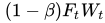
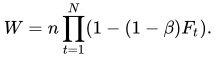
After round ${\displaystyle t}$, the total weight is decreased by${\displaystyle \ (1-\beta )F_{t}W_{t}}$, since all weights corresponding to a wrong answer are multiplied by${\displaystyle \ \beta <1}$. It then follows that ${\displaystyle W_{t+1}=W_{t}(1-(1-\beta )F_{t})}$. By telescoping, since ${\displaystyle W_{1}=n}$, it follows that the total weight after the process concludes is

${\displaystyle {\begin{aligned}W=n\prod _{t=1}^{N}(1-(1-\beta )F_{t}).\end{aligned}}}$

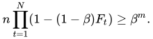
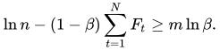
On the other hand, suppose that ${\displaystyle \ m}$ is the number of mistakes made by the best-performing expert. At the end, this expert has weight ${\displaystyle \ \beta ^{m}}$. It follows, then, that the total weight is at least this much; in other words, ${\displaystyle \ W\geq \beta ^{m}}$. This inequality and the above result imply

${\displaystyle {\begin{aligned}n\prod _{t=1}^{N}(1-(1-\beta )F_{t})\geq \beta ^{m}.\end{aligned}}}$

Taking the natural logarithm of both sides yields

${\displaystyle {\begin{aligned}\ln n+\sum _{t=1}^{N}\ln(1-(1-\beta )F_{t})\geq m\ln \beta .\end{aligned}}}$

Now, the Taylor series of the natural logarithm is

${\displaystyle {\begin{aligned}\ln(1-x)=-x-{\frac {x^{2}}{2}}-{\frac {x^{3}}{3}}-\cdots \end{aligned}}}$

In particular, it follows that${\displaystyle \ \ln(1-(1-\beta )F_{t})<-(1-\beta )F_{t}}$.
Thus,

${\displaystyle {\begin{aligned}\ln n-(1-\beta )\sum _{t=1}^{N}F_{t}\geq m\ln \beta .\end{aligned}}}$

Recalling that ${\displaystyle E[M]=\sum _{t=1}^{N}F_{t}}$ and rearranging, it follows that

${\displaystyle {\begin{aligned}E[M]\leq {\frac {m\ln(1/\beta )+\ln(n)}{1-\beta }}={\frac {\ln(1/\beta )}{1-\beta }}m+{\frac {1}{1-\beta }}\ln(n).\end{aligned}}}$

Now, as ${\displaystyle \beta \to 1}$ from below, the first constant tends to ${\displaystyle 1}$; however, the second constant tends to ${\displaystyle +\infty }$. To quantify this tradeoff, define ${\displaystyle \varepsilon =1-\beta }$ to be the penalty associated with getting a prediction wrong. Then, again applying the Taylor series of the natural logarithm,

${\displaystyle {\begin{aligned}{\frac {\ln(1/\beta )}{1-\beta }}=-{\frac {\ln(\beta )}{1-\beta }}={\frac {-\ln(1-\varepsilon )}{\varepsilon }}={\frac {\varepsilon +{\frac {\varepsilon ^{2}}{2}}+{\frac {\varepsilon ^{3}}{3}}+\cdots }{\varepsilon }}=1+{\frac {\varepsilon }{2}}+O(\varepsilon ^{2})\end{aligned}}}$

It then follows that the mistake bound, for small ${\displaystyle \varepsilon }$, can be written in the form ${\displaystyle \ \left(1+{\frac {\epsilon }{2}}+O(\varepsilon ^{2})\right)m+\epsilon ^{-1}\ln(n)}$.

In English, the less that we penalize experts for their mistakes, the more that additional experts will lead to initial mistakes but the closer we get to capturing the predictive accuracy of the best expert as time goes on. In particular, given a sufficiently low value of ${\displaystyle \varepsilon }$ and enough rounds, the randomized weighted majority algorithm can get arbitrarily close to the correct prediction rate of the best expert.

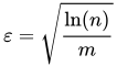
In particular, as long as ${\displaystyle m}$ is sufficiently large compared to ${\displaystyle \ln(n)}$ (so that their ratio is sufficiently small), we can assign

${\displaystyle {\begin{aligned}\varepsilon ={\sqrt {\frac {\ln(n)}{m}}}\end{aligned}}}$

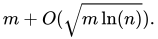
we can obtain an upper bound on the number of mistakes equal to

${\displaystyle {\begin{aligned}m+O({\sqrt {m\ln(n)}}).\end{aligned}}}$

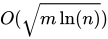
This implies that the "regret bound" on the algorithm (that is, how much worse it performs than the best expert) is sublinear, at ${\displaystyle O({\sqrt {m\ln(n)}})}$.

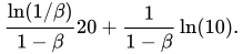
Recall that the motivation for the randomized weighted majority algorithm was given by an example where the best expert makes a mistake 20% of the time. Precisely, in ${\displaystyle N=100}$ rounds, with ${\displaystyle n=10}$ experts, where the best expert makes ${\displaystyle m=20}$ mistakes, the deterministic weighted majority algorithm only guarantees an upper bound of ${\displaystyle 2.4(\log _{2}10+20)\approx 56}$. By the analysis above, it follows that minimizing the number of worst-case expected mistakes is equivalent to minimizing the function

${\displaystyle {\begin{aligned}{\frac {\ln(1/\beta )}{1-\beta }}20+{\frac {1}{1-\beta }}\ln(10).\end{aligned}}}$

Computational methods show that the optimal value is roughly ${\displaystyle \beta \approx 0.641}$, which results in the minimal worst-case number of expected mistakes of ${\displaystyle E[M]\approx 31.19}$. When the number of rounds is increased (say, to ${\displaystyle N=1000000}$) while the accuracy rate of the best expert is kept the same the improvement can be even more dramatic; the weighted majority algorithm guarantees only a worst-case mistake rate of 48.0%, but the randomized weighted majority algorithm, when properly tuned to the optimal value of ${\displaystyle \varepsilon \approx 0.0117}$, achieves a worst-case mistake rate of 20.2%.

The Randomized Weighted Majority Algorithm can be used to combine multiple algorithms in which case RWMA can be expected to perform nearly as well as the best of the original algorithms in hindsight. Note that the RWMA can be generalized to solve problems which do not have binary mistake variables, which makes it useful for a wide class of problems.

Furthermore, one can apply the Randomized Weighted Majority Algorithm in situations where experts are making choices that cannot be combined (or can't be combined easily). For example, RWMA can be applied to repeated game-playing or the online shortest path problem. In the online shortest path problem, each expert is telling you a different way to drive to work. You pick one path using RWMA. Later you find out how well you would have done using all of the suggested paths and penalize appropriately. The goal is to have an expected loss not much larger than the loss of the best expert.

The randomized weighted majority algorithm has been proposed as a new method for several practical software applications, particularly in the domains of bug detection and cyber-security.^[3][4] For instance, Varsha and Madhavu (2021) describe how the randomized weighted majority algorithm can be used to replace conventional voting within a random forest classification approach to detect insider threats. Using experimental results, they show that this approach obtained a higher level of accuracy and recall compared to the standard random forest algorithm. Moustafa et al. (2018) have studied how an ensemble classifier based on the randomized weighted majority algorithm could be used to detect bugs earlier in the software development process, after being trained on existing software repositories.

• Multi-armed bandit problem.
• Efficient algorithm for some cases with many experts.
• Sleeping experts/"specialists" setting.

• Machine learning
• Weighted majority algorithm
• Game theory
• Multi-armed bandit

• Weighted Majority & Randomized Weighted Majority
• Avrim Blum (2004) machine learning theory
• Rob Schapire 2006 Foundations of Machine Learning
• Predicting From Experts Advice
• Uri Feige, Robi Krauthgamer, Moni Naor. Algorithmic Game Theory
• Nika Haghtalab 2020 Theoretical Foundations of Machine Learning (Notes)