Explore Black History

In statistics, a rank correlation is any of several statistics that measure an ordinal association — the relationship between rankings of different ordinal variables or different rankings of the same variable, where a "ranking" is the assignment of the ordering labels "first", "second", "third", etc. to different observations of a particular variable. A rank correlation coefficient measures the degree of similarity between two rankings, and can be used to assess the significance of the relation between them. For example, two common nonparametric methods of significance that use rank correlation are the Mann–Whitney U test and the Wilcoxon signed-rank test.

If, for example, one variable is the identity of a college basketball program and another variable is the identity of a college football program, one could test for a relationship between the poll rankings of the two types of program: do colleges with a higher-ranked basketball program tend to have a higher-ranked football program? A rank correlation coefficient can measure that relationship, and the measure of significance of the rank correlation coefficient can show whether the measured relationship is small enough to likely be a coincidence.

If there is only one variable, the identity of a college football program, but it is subject to two different poll rankings (say, one by coaches and one by sportswriters), then the similarity of the two different polls' rankings can be measured with a rank correlation coefficient.

As another example, in a contingency table with low income, medium income, and high income in the row variable and educational level—no high school, high school, university—in the column variable,^[1] a rank correlation measures the relationship between income and educational level.

Some of the more popular rank correlation statistics include

1. Spearman's ρ
2. Kendall's τ
3. Goodman and Kruskal's γ
4. Somers' D

An increasing rank correlation coefficient implies increasing agreement between rankings. The coefficient is inside the interval [−1, 1] and assumes the value:

• 1 if the agreement between the two rankings is perfect; the two rankings are the same.
• 0 if the rankings are completely independent.
• −1 if the disagreement between the two rankings is perfect; one ranking is the reverse of the other.

Following Diaconis (1988), a ranking can be seen as a permutation of a set of objects. Thus we can look at observed rankings as data obtained when the sample space is (identified with) a symmetric group. We can then introduce a metric, making the symmetric group into a metric space. Different metrics will correspond to different rank correlations.

Kendall 1970^[2] showed that his ${\displaystyle \tau }$ (tau) and Spearman's ${\displaystyle \rho }$ (rho) are particular cases of a general correlation coefficient.

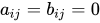
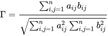
Suppose we have a set of ${\displaystyle n}$ objects, which are being considered in relation to two properties, represented by ${\displaystyle x}$ and ${\displaystyle y}$, forming the sets of values ${\displaystyle \{x_{i}\}_{i\leq n}}$ and ${\displaystyle \{y_{i}\}_{i\leq n}}$. To any pair of individuals, say the ${\displaystyle i}$-th and the ${\displaystyle j}$-th we assign a ${\displaystyle x}$-score, denoted by ${\displaystyle a_{ij}}$, and a ${\displaystyle y}$-score, denoted by ${\displaystyle b_{ij}}$. The only requirement for these functions is that they be anti-symmetric, so ${\displaystyle a_{ij}=-a_{ji}}$ and ${\displaystyle b_{ij}=-b_{ji}}$. (Note that in particular ${\displaystyle a_{ij}=b_{ij}=0}$ if ${\displaystyle i=j}$.) Then the generalized correlation coefficient ${\displaystyle \Gamma }$ is defined as

${\displaystyle \Gamma ={\frac {\sum _{i,j=1}^{n}a_{ij}b_{ij}}{\sqrt {\sum _{i,j=1}^{n}a_{ij}^{2}\sum _{i,j=1}^{n}b_{ij}^{2}}}}}$

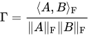
Equivalently, if all coefficients are collected into matrices ${\displaystyle A=(a_{ij})}$ and ${\displaystyle B=(b_{ij})}$, with ${\displaystyle A^{\textsf {T}}=-A}$ and ${\displaystyle B^{\textsf {T}}=-B}$, then

${\displaystyle \Gamma ={\frac {\langle A,B\rangle _{\rm {F}}}{\|A\|_{\rm {F}}\|B\|_{\rm {F}}}}}$

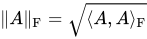
where ${\displaystyle \langle A,B\rangle _{\rm {F}}}$ is the Frobenius inner product and ${\displaystyle \|A\|_{\rm {F}}={\sqrt {\langle A,A\rangle _{\rm {F}}}}}$ the Frobenius norm. In particular, the general correlation coefficient is the cosine of the angle between the matrices ${\displaystyle A}$ and ${\displaystyle B}$.

If ${\displaystyle r_{i}}$, ${\displaystyle s_{i}}$ are the ranks of the ${\displaystyle i}$-member according to the ${\displaystyle x}$-quality and ${\displaystyle y}$-quality respectively, then we can define

${\displaystyle a_{ij}=\operatorname {sgn}(r_{j}-r_{i}),\quad b_{ij}=\operatorname {sgn}(s_{j}-s_{i}).}$

The sum ${\displaystyle \sum a_{ij}b_{ij}}$ is the number of concordant pairs minus the number of discordant pairs (see Kendall tau rank correlation coefficient). The sum ${\displaystyle \sum a_{ij}^{2}}$ is just ${\displaystyle n(n-1)/2}$, the number of terms ${\displaystyle a_{ij}}$, as is ${\displaystyle \sum b_{ij}^{2}}$. Thus in this case,

${\displaystyle \Gamma ={\frac {2\,(({\text{number of concordant pairs}})-({\text{number of discordant pairs}}))}{n(n-1)}}={\text{Kendall's }}\tau }$

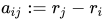
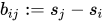
If ${\displaystyle r_{i}}$, ${\displaystyle s_{i}}$ are the ranks of the ${\displaystyle i}$-member according to the ${\displaystyle x}$ and the ${\displaystyle y}$-quality respectively, we may consider the matrices ${\displaystyle a,b\in M(n\times n;\mathbb {R} )}$ defined by

${\displaystyle a_{ij}:=r_{j}-r_{i}}$

${\displaystyle b_{ij}:=s_{j}-s_{i}}$

The sums ${\displaystyle \sum a_{ij}^{2}}$ and ${\displaystyle \sum b_{ij}^{2}}$ are equal, since both ${\displaystyle r_{i}}$ and ${\displaystyle s_{i}}$ range from ${\displaystyle 1}$ to ${\displaystyle n}$. Hence

${\displaystyle \Gamma ={\frac {\sum (r_{j}-r_{i})(s_{j}-s_{i})}{\sum (r_{j}-r_{i})^{2}}}}$

To simplify this expression, let ${\displaystyle d_{i}:=r_{i}-s_{i}}$ denote the difference in the ranks for each ${\displaystyle i}$. Further, let ${\displaystyle U}$ be a uniformly distributed discrete random variables on ${\displaystyle \{1,2,\ldots ,n\}}$. Since the ranks ${\displaystyle r,s}$ are just permutations of ${\displaystyle 1,2,\ldots ,n}$, we can view both as being random variables distributed like ${\displaystyle U}$. Using basic summation results from discrete mathematics, it is easy to see that for the uniformly distributed random variable, ${\displaystyle U}$, we have ${\displaystyle \mathbb {E} [U]=\textstyle {\frac {n+1}{2}}}$ and ${\displaystyle \mathbb {E} [U^{2}]=\textstyle {\frac {(n+1)(2n+1)}{6}}}$ and thus ${\displaystyle \mathrm {Var} (U)=\textstyle {\frac {(n+1)(2n+1)}{6}}-\textstyle {\frac {(n+1)(n+1)}{4}}=\textstyle {\frac {n^{2}-1}{12}}}$. Now, observing symmetries allows us to compute the parts of ${\displaystyle \Gamma }$ as follows:

${\displaystyle {\begin{aligned}{\frac {1}{n^{2}}}\sum _{i,j=1}^{n}(r_{j}-r_{i})(s_{j}-s_{i})&=2\left({\frac {1}{n^{2}}}\cdot n\sum _{i=1}^{n}r_{i}s_{i}-\left({\frac {1}{n}}\sum _{i=1}^{n}r_{i}\right)\left({\frac {1}{n}}\sum _{j=1}^{n}s_{j}\right)\right)\\&={\frac {1}{n}}\sum _{i=1}^{n}(r_{i}^{2}+s_{i}^{2}-d_{i}^{2})-2\left(\mathbb {E} [U]\right)^{2}\\&={\frac {1}{n}}\sum _{i=1}^{n}r_{i}^{2}+{\frac {1}{n}}\sum _{i=1}^{n}s_{i}^{2}-{\frac {1}{n}}\sum _{i=1}^{n}d_{i}^{2}-2\left(\mathbb {E} [U]\right)^{2}\\&=2\left(\mathbb {E} [U^{2}]-(\mathbb {E} [U])^{2}\right)-{\frac {1}{n}}\sum _{i=1}^{n}d_{i}^{2}\\\end{aligned}}}$

and

${\displaystyle {\begin{aligned}{\frac {1}{n^{2}}}\sum _{i,j=1}^{n}(r_{j}-r_{i})^{2}&={\frac {1}{n^{2}}}\cdot n\sum _{i,j=1}^{n}(r_{i}^{2}+r_{j}^{2}-2r_{i}r_{j})\\&=2{\frac {1}{n}}\sum _{i=1}^{n}r_{i}^{2}-2\left({\frac {1}{n}}\sum _{i=1}^{n}r_{i}\right)\left({\frac {1}{n}}\sum _{j=1}^{n}r_{j}\right)\\&=2(\mathbb {E} [U^{2}]-(\mathbb {E} [U])^{2})\\\end{aligned}}}$

Hence

${\displaystyle \Gamma =1-{\frac {\sum _{i=1}^{n}d_{i}^{2}}{2n\mathrm {Var} (U)}}=1-{\frac {6\sum _{i=1}^{n}d_{i}^{2}}{n(n^{2}-1)}}}$

where ${\displaystyle d_{i}=r_{i}-s_{i}}$ is the difference between ranks, which is exactly Spearman's rank correlation coefficient ${\displaystyle \rho }$.

Gene Glass (1965) noted that the rank-biserial can be derived from Spearman's ${\displaystyle \rho }$. "One can derive a coefficient defined on X, the dichotomous variable, and Y, the ranking variable, which estimates Spearman's rho between X and Y in the same way that biserial r estimates Pearson's r between two normal variables" (p. 91). The rank-biserial correlation had been introduced nine years before by Edward Cureton (1956) as a measure of rank correlation when the ranks are in two groups.^[3]

Dave Kerby (2014) recommended the rank-biserial as the measure to introduce students to rank correlation, because the general logic can be explained at an introductory level. The rank-biserial is the correlation used with the Mann–Whitney U test, a method commonly covered in introductory college courses on statistics. The data for this test consists of two groups; and for each member of the groups, the outcome is ranked for the study as a whole.

Kerby showed that this rank correlation can be expressed in terms of two concepts: the percent of data that support a stated hypothesis, and the percent of data that do not support it. The Kerby simple difference formula states that the rank correlation can be expressed as the difference between the proportion of favorable evidence (f) minus the proportion of unfavorable evidence (u).

${\displaystyle r=f-u}$

To illustrate the computation, suppose a coach trains long-distance runners for one month using two methods. Group A has 5 runners, and Group B has 4 runners. The stated hypothesis is that method A produces faster runners. The race to assess the results finds that the runners from Group A do indeed run faster, with the following ranks: 1, 2, 3, 4, and 6. The slower runners from Group B thus have ranks of 5, 7, 8, and 9.

The analysis is conducted on pairs, defined as a member of one group compared to a member of the other group. For example, the fastest runner in the study is a member of four pairs: (1,5), (1,7), (1,8), and (1,9). All four of these pairs support the hypothesis, because in each pair the runner from Group A is faster than the runner from Group B. There are a total of 20 pairs, and 19 pairs support the hypothesis. The only pair that does not support the hypothesis are the two runners with ranks 5 and 6, because in this pair, the runner from Group B had the faster time. By the Kerby simple difference formula, 95% of the data support the hypothesis (19 of 20 pairs), and 5% do not support (1 of 20 pairs), so the rank correlation is r = .95 − .05 = .90.

The maximum value for the correlation is r = 1, which means that 100% of the pairs favor the hypothesis. A correlation of r = 0 indicates that half the pairs favor the hypothesis and half do not; in other words, the sample groups do not differ in ranks, so there is no evidence that they come from two different populations. An effect size of r = 0 can be said to describe no relationship between group membership and the members' ranks.

In their article “Improving statistical reporting in psychology,” Anna-Lena Schubert and her colleagues (2025) set forth guidelines for statistical reporting, drawing from established recommendations and emerging best practices. In Table 5 they offered an overview of effect sizes for commonly used statistical models. In this table they cited the Kerby (2014) paper as a key resource for the application and interpretation of the rank-biserial correlation.

• Cureton, Edward E. (1956). "Rank-biserial correlation". Psychometrika. 21 (3): 287–290. doi:10.1007/BF02289138. S2CID 122500836.
• Everitt, B. S. (2002), The Cambridge Dictionary of Statistics, Cambridge: Cambridge University Press, ISBN 0-521-81099-X
• Diaconis, P. (1988), Group Representations in Probability and Statistics, Lecture Notes-Monograph Series, Hayward, CA: Institute of Mathematical Statistics, ISBN 0-940600-14-5
• Glass, Gene V. (1965). "A ranking variable analogue of biserial correlation: implications for short-cut item analysis". Journal of Educational Measurement. 2 (1): 91–95. doi:10.1111/j.1745-3984.1965.tb00396.x.
• Kendall, M. G. (1970), Rank Correlation Methods, London: Griffin, ISBN 0-85264-199-0
• Kerby, Dave S. (2014). "The Simple Difference Formula: An Approach to Teaching Nonparametric Correlation". Comprehensive Psychology. 3 (1) 11.IT.3.1. doi:10.2466/11.IT.3.1.
• Schubert, A.L.; Steinhilber, M.; Kang, H.; Quintana, D.S. (2025). "Improving statistical reporting in psychology". Communications Psychology. 3 (1) 156. doi:10.1038/s44271-025-00356-w. PMC 12618885. PMID 41238797.

• Brief guide by experimental psychologist Karl L. Weunsch - Nonparametric effect sizes (Copyright 2015 by Karl L. Weunsch)