Explore Black History

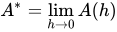
In numerical analysis, Richardson extrapolation is a method used to estimate some value ${\displaystyle A^{\ast }=\lim _{h\to 0}A(h)}$ if the truncation error is known to have a (possibly 1-sided) power-series expansion at ${\displaystyle h=0}$. The method is most often applied as a sequence acceleration method to improve the rate of convergence of iterative methods. It is named after Lewis Fry Richardson, who introduced the technique in the early 20th century,^[1][2] though a form of the idea was already known to Christiaan Huygens in the 17th century and used his calculation of ${\displaystyle \pi }$.^[3] Practical applications of Richardson extrapolation include Romberg integration, which applies Richardson extrapolation to the trapezoid rule, and the Bulirsch–Stoer algorithm for solving ordinary differential equations. In the words of Birkhoff and Rota, "its usefulness for practical computations can hardly be overestimated."^[4]

Let ${\displaystyle A_{0}(h)}$ be an approximation of ${\displaystyle A^{*}}$(exact value) that depends on a step size h (where ${\textstyle 0<h<1}$) with an error formula of the form $${\displaystyle A^{*}-A_{0}(h)=a_{0}h^{k_{0}}+a_{1}h^{k_{1}}+a_{2}h^{k_{2}}+\cdots }$$ where the ${\displaystyle a_{i}}$ are unknown constants and the ${\displaystyle k_{i}}$ are known constants such that ${\displaystyle h^{k_{i}}>h^{k_{i+1}}}$. Furthermore, ${\displaystyle O(h^{k_{i}})}$ represents the truncation error of the ${\displaystyle A_{i}(h)}$ approximation such that ${\displaystyle A^{*}-A_{i}(h)=O(h^{k_{i}}).}$ Note that by simplifying with Big O notation, the following asymptotic formulae are implied: $${\displaystyle {\begin{aligned}A^{*}-A_{0}(h)&=a_{0}h^{k_{0}}+a_{1}h^{k_{1}}+a_{2}h^{k_{2}}+\cdots \\&=a_{0}h^{k_{0}}+O{\left(h^{k_{1}}\right)}\\&=O{\left(h^{k_{0}}\right)}\end{aligned}}}$$

Richardson extrapolation is a process that finds a better approximation of ${\displaystyle A^{*}}$ by changing the error formula from ${\displaystyle A^{*}=A_{0}(h)+O(h^{k_{0}})}$ to ${\displaystyle A^{*}=A_{1}(h)+O(h^{k_{1}}).}$ Therefore, by replacing ${\displaystyle A_{0}(h)}$ with ${\displaystyle A_{1}(h)}$ the truncation error has reduced from ${\displaystyle O(h^{k_{0}})}$ to ${\displaystyle O(h^{k_{1}})}$ for the same step size ${\displaystyle h}$. The general pattern occurs in which ${\displaystyle A_{i}(h)}$ is a more accurate estimate than ${\displaystyle A_{j}(h)}$ when ${\displaystyle i>j}$. By this process, we have achieved a better approximation of ${\displaystyle A^{*}}$ by subtracting the largest term in the error which was ${\displaystyle O(h^{k_{0}})}$. This process can be repeated to remove more error terms to get even better approximations.

Using the step sizes ${\displaystyle h}$ and ${\displaystyle h/t}$ for some constant ${\displaystyle t}$, the two formulas for ${\displaystyle A^{*}}$ are:

$${\displaystyle A^{*}=A_{0}(h)+a_{0}h^{k_{0}}+a_{1}h^{k_{1}}+a_{2}h^{k_{2}}+O(h^{k_{3}})}$$

1

$${\displaystyle A^{*}=A_{0}\!\left({\frac {h}{t}}\right)+a_{0}\left({\frac {h}{t}}\right)^{k_{0}}+a_{1}\left({\frac {h}{t}}\right)^{k_{1}}+a_{2}\left({\frac {h}{t}}\right)^{k_{2}}+O(h^{k_{3}})}$$

2

To improve our approximation from ${\displaystyle O(h^{k_{0}})}$ to ${\displaystyle O(h^{k_{1}})}$ by removing the first error term, we multiply equation 2 by ${\displaystyle t^{k_{0}}}$ and subtract equation 1 to give us $${\displaystyle (t^{k_{0}}-1)A^{*}=\left[t^{k_{0}}A_{0}{\left({\frac {h}{t}}\right)}-A_{0}(h)\right]+\left[t^{k_{0}}a_{1}\left({\frac {h}{t}}\right)^{k_{1}}-a_{1}h^{k_{1}}\right]+\left[t^{k_{0}}a_{2}\left({\frac {h}{t}}\right)^{k_{2}}-a_{2}h^{k_{2}}\right]+O{\left(h^{k_{3}}\right)}.}$$ This multiplication and subtraction was performed because ${\textstyle {\big [}t^{k_{0}}A_{0}\left({\frac {h}{t}}\right)-A_{0}(h){\big ]}}$ is an ${\displaystyle O(h^{k_{1}})}$ approximation of ${\displaystyle (t^{k_{0}}-1)A^{*}}$. We can solve our current formula for ${\displaystyle A^{*}}$ to give $${\displaystyle A^{*}={\frac {t^{k_{0}}A_{0}{\left({\frac {h}{t}}\right)}-A_{0}(h)}{t^{k_{0}}-1}}+{\frac {t^{k_{0}}a_{1}\left({\frac {h}{t}}\right)^{k_{1}}-a_{1}h^{k_{1}}}{t^{k_{0}}-1}}+{\frac {t^{k_{0}}a_{2}\left({\frac {h}{t}}\right)^{k_{2}}-a_{2}h^{k_{2}}}{t^{k_{0}}-1}}+O{\left(h^{k_{3}}\right)}}$$ which can be written as ${\displaystyle A^{*}=A_{1}(h)+O(h^{k_{1}})}$ by setting $${\displaystyle A_{1}(h)={\frac {t^{k_{0}}A_{0}{\left({\frac {h}{t}}\right)}-A_{0}(h)}{t^{k_{0}}-1}}.}$$

A general recurrence relation can be defined for the approximations by $${\displaystyle A_{i+1}(h)={\frac {t^{k_{i}}A_{i}{\left({\frac {h}{t}}\right)}-A_{i}(h)}{t^{k_{i}}-1}}}$$ where ${\displaystyle k_{i+1}}$ satisfies $${\displaystyle A^{*}=A_{i+1}(h)+O(h^{k_{i+1}}).}$$

The Richardson extrapolation can be considered as a linear sequence transformation.

Additionally, the general formula can be used to estimate ${\displaystyle k_{0}}$ (leading order step size behavior of Truncation error) when neither its value nor ${\displaystyle A^{*}}$ is known a priori. Such a technique can be useful for quantifying an unknown rate of convergence. Given approximations of ${\displaystyle A^{*}}$ from three distinct step sizes ${\displaystyle h}$, ${\displaystyle h/t}$, and ${\displaystyle h/s}$, the exact relationship $${\displaystyle {\begin{aligned}A^{*}&={\frac {t^{k_{0}}A_{i}{\left({\frac {h}{t}}\right)}-A_{i}(h)}{t^{k_{0}}-1}}+O{\left(h^{k_{1}}\right)}\\[1ex]&={\frac {s^{k_{0}}A_{i}{\left({\frac {h}{s}}\right)}-A_{i}(h)}{s^{k_{0}}-1}}+O{\left(h^{k_{1}}\right)}\end{aligned}}}$$ yields an approximate relationship (please note that the notation here may cause a bit of confusion, the two O appearing in the equation above only indicates the leading order step size behavior but their explicit forms are different and hence cancelling out of the two O terms is only approximately valid) $${\displaystyle A_{i}{\left({\frac {h}{t}}\right)}+{\frac {A_{i}{\left({\frac {h}{t}}\right)}-A_{i}(h)}{t^{k_{0}}-1}}\approx A_{i}{\left({\frac {h}{s}}\right)}+{\frac {A_{i}{\left({\frac {h}{s}}\right)}-A_{i}(h)}{s^{k_{0}}-1}}}$$ which can be solved numerically to estimate ${\displaystyle k_{0}}$ for some arbitrary valid choices of ${\displaystyle h}$, ${\displaystyle s}$, and ${\displaystyle t}$.

As ${\displaystyle t\neq 1}$, if ${\displaystyle t>0}$ and ${\displaystyle s}$ is chosen so that ${\displaystyle s=t^{2}}$, this approximate relation reduces to a quadratic equation in ${\displaystyle t^{k_{0}}}$, which is readily solved for ${\displaystyle k_{0}}$ in terms of ${\displaystyle h}$ and ${\displaystyle t}$.

Suppose that we wish to approximate ${\displaystyle A^{*}}$, and we have a method ${\displaystyle A(h)}$ that depends on a small parameter ${\displaystyle h}$ in such a way that $${\displaystyle A(h)=A^{\ast }+Ch^{n}+O(h^{n+1}).}$$

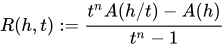
Let us define a new function$${\displaystyle R(h,t):={\frac {t^{n}A(h/t)-A(h)}{t^{n}-1}}}$$where ${\displaystyle h}$ and ${\displaystyle {\frac {h}{t}}}$ are two distinct step sizes.

Then $${\displaystyle {\begin{aligned}R(h,t)&={\frac {t^{n}\left[A^{*}+C\left({\frac {h}{t}}\right)^{n}+O{\left(h^{n+1}\right)}\right]-\left[A^{*}+Ch^{n}+O{\left(h^{n+1}\right)}\right]}{t^{n}-1}}\\&=A^{*}+O{\left(h^{n+1}\right)}.\end{aligned}}}$$ ${\displaystyle R(h,t)}$ is called the Richardson extrapolation of A(h), and has a higher-order error estimate ${\displaystyle O(h^{n+1})}$ compared to ${\displaystyle A(h)}$.

Very often, it is much easier to obtain a given precision by using R(h) rather than A(h′) with a much smaller h′. Where A(h′) can cause problems due to limited precision (rounding errors) and/or due to the increasing number of calculations needed (see examples below).

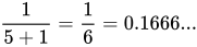
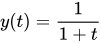
The following pseudocode in MATLAB style demonstrates Richardson extrapolation to help solve the ODE ${\displaystyle y'(t)=-y^{2}}$, ${\displaystyle y(0)=1}$ with the Trapezoidal method. In this example we halve the step size ${\displaystyle h}$ each iteration and so in the discussion above we'd have that ${\displaystyle t=2}$. The error of the Trapezoidal method can be expressed in terms of odd powers so that the error over multiple steps can be expressed in even powers; this leads us to raise ${\displaystyle t}$ to the second power and to take powers of ${\displaystyle 4=2^{2}=t^{2}}$ in the pseudocode. We want to find the value of ${\displaystyle y(5)}$, which has the exact solution of ${\displaystyle {\frac {1}{5+1}}={\frac {1}{6}}=0.1666...}$ since the exact solution of the ODE is ${\displaystyle y(t)={\frac {1}{1+t}}}$. This pseudocode assumes that a function called Trapezoidal(f, tStart, tEnd, h, y0) exists which attempts to compute y(tEnd) by performing the trapezoidal method on the function f, with starting point y0 and tStart and step size h.

Note that starting with too small an initial step size can potentially introduce error into the final solution. Although there are methods designed to help pick the best initial step size, one option is to start with a large step size and then to allow the Richardson extrapolation to reduce the step size each iteration until the error reaches the desired tolerance.

tStart = 0          % Starting time
tEnd = 5            % Ending time
f = -y^2            % The derivative of y, so y' = f(t, y(t)) = -y^2
                    % The solution to this ODE is y = 1/(1 + t)
y0 = 1              % The initial position (i.e. y0 = y(tStart) = y(0) = 1)
tolerance = 10^-11  % 10 digit accuracy is desired

% Don't allow the iteration to continue indefinitely
maxRows = 20
% Pick an initial step size
initialH = tStart - tEnd
% Were we able to find the solution to within the desired tolerance? not yet.
haveWeFoundSolution = false

h = initialH

% Create a 2D matrix of size maxRows by maxRows to hold the Richardson extrapolates
% Note that this will be a lower triangular matrix and that at most two rows are actually
% needed at any time in the computation.
A = zeroMatrix(maxRows, maxRows)

% Compute the top left element of the matrix.
% The first row of this (lower triangular) matrix has now been filled.
A(1, 1) = Trapezoidal(f, tStart, tEnd, h, y0)

% Each row of the matrix requires one call to Trapezoidal
% This loops starts by filling the second row of the matrix,
% since the first row was computed above
for i = 1 : maxRows - 1 % Starting at i = 1, iterate at most maxRows - 1 times
    % Halve the previous value of h since this is the start of a new row.
    h = h/2

    % Starting filling row i+1 from the left by calling
    % the Trapezoidal function with this new smaller step size
    A(i + 1, 1) = Trapezoidal(f, tStart, tEnd, h, y0)

    % Go across this current (i+1)-th row until the diagonal is reached
    for j = 1 : i
        % To compute A(i + 1, j + 1), which is the next Richardson extrapolate, 
        % use the most recently computed value (i.e. A(i + 1, j))
        % and the value from the row above it (i.e. A(i, j)).

        A(i + 1, j + 1) = ((4^j).*A(i + 1, j) - A(i, j))/(4^j - 1);
    end
    
    % After leaving the above inner loop, the diagonal element of row i + 1 has been computed
    % This diagonal element is the latest Richardson extrapolate to be computed.
    % The difference between this extrapolate and the last extrapolate of row i is a good
    % indication of the error.
    if (absoluteValue(A(i + 1, i + 1) - A(i, i)) < tolerance)  % If the result is within tolerance
        % Display the result of the Richardson extrapolation
        print("y = ", A(i + 1, i + 1))
        haveWeFoundSolution = true
        % Done, so leave the loop
        break
    end
end

% If we were not able to find a solution to within the desired tolerance
if (not haveWeFoundSolution)
    print("Warning: Not able to find solution to within the desired tolerance of ", tolerance);
    print("The last computed extrapolate was ", A(maxRows, maxRows))
end

• Aitken's delta-squared process
• Takebe Kenko
• Richardson iteration

• Feldman, Joel (2000). "Richardson-Extrapolation" (PDF).
• Israel, Robert. "Richardson extrapolation".
• Matlab code for generic Richardson extrapolation.
• Julia code for generic Richardson extrapolation.