Explore Black History

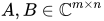
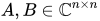
In mathematics, in particular in functional analysis, the singular values of a compact operator ${\displaystyle \,T\!:X\rightarrow Y}$ acting between Hilbert spaces ${\displaystyle X}$ and ⁠${\displaystyle Y}$⁠, are the square roots of the (necessarily non-negative) eigenvalues of the self-adjoint operator ${\displaystyle T^{*}T}$ (where ${\displaystyle T^{*}}$ denotes the adjoint of ⁠${\displaystyle T}$⁠).

The singular values are non-negative real numbers, usually listed in decreasing order ⁠${\displaystyle {\big (}\sigma _{1}(T)\geq \sigma _{2}(T)\geq \dots {\big )}}$⁠. The largest singular value ${\displaystyle \sigma _{1}(T)}$ is equal to the operator norm of ${\displaystyle T}$ (see Min-max theorem).

If ${\displaystyle T}$ acts on a Euclidean space (for example, ⁠${\displaystyle \mathbb {R} ^{n}}$⁠), there is a simple geometric interpretation for the singular values: Consider the image by ${\displaystyle T}$ of the unit sphere; this is an ellipsoid, and the lengths of its semi-axes are the singular values of ${\displaystyle T}$ (the figure provides an example in ⁠${\displaystyle \mathbb {R} ^{2}}$⁠).

If ⁠${\displaystyle A}$⁠ is a normal matrix, then its singular values are the absolute values of its eigenvalues. Indeed, in this case, the spectral theorem can be applied to obtain unitary diagonalization of ${\displaystyle A}$ as ⁠${\displaystyle A=U\varLambda \,U^{*}}$⁠. Then, by definition, ⁠${\displaystyle \textstyle {\sqrt {A^{*}A}}=U{\sqrt {\varLambda ^{*}\varLambda }}~U^{*}=U\,\vert \varLambda \vert ~U^{*}}$⁠.

Most norms on Hilbert space operators studied are defined using singular values. For example, the Ky Fan ⁠${\displaystyle k}$⁠-norm is the sum of the first ${\displaystyle k}$ singular values, the trace norm is the sum of all singular values, and the Schatten norm is the ⁠${\displaystyle p}$⁠-th root of the sum of the ⁠${\displaystyle p}$⁠-th powers of the singular values. Note that each norm is defined only on a special class of operators, hence singular values can be useful in classifying different operators.

In the finite-dimensional case, a matrix can always be decomposed in the form ⁠${\displaystyle U\varSigma \,V^{*}}$⁠, where ${\displaystyle U}$ and ${\displaystyle V^{*}}$ are unitary matrices and ${\displaystyle \varSigma }$ is a rectangular diagonal matrix with the singular values lying on its diagonal. This is the singular value decomposition.

For ${\displaystyle A\in \mathbb {C} ^{m\times n}}$ and ⁠${\displaystyle i=1,2,\ldots ,\min\{m,n\}}$⁠:

Min-max theorem for singular values:
Here, ${\displaystyle U}$ is a subspace of ⁠${\displaystyle \mathbb {C} ^{n}}$⁠;

${\displaystyle \sigma _{i}(A)=\min _{\dim(U)=n-i+1}\max _{\underset {\|x\|_{2}=1}{x\in U}}\left\|Ax\right\|_{2}.}$

${\displaystyle \sigma _{i}(A)=\max _{\dim(U)=i}\min _{\underset {\|x\|_{2}=1}{x\in U}}\left\|Ax\right\|_{2}.}$

Matrix transpose and conjugate do not alter singular values:

⁠${\displaystyle \sigma _{i}(A)=\sigma _{i}\!\left(A^{\textsf {T}}\right)=\sigma _{i}\!\left(A^{*}\right)}$⁠.

For any unitary matrices ${\displaystyle U\in \mathbb {C} ^{m\times m}}$ and ⁠${\displaystyle V\in \mathbb {C} ^{n\times n}}$⁠,

⁠${\displaystyle \sigma _{i}(A)=\sigma _{i}(UAV)}$⁠.

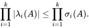
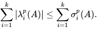
Relation to eigenvalues:

⁠${\displaystyle \sigma _{i}^{2}(A)=\lambda _{i}\!\left(AA^{*}\right)=\lambda _{i}\!\left(A^{*}A\right)}$⁠.

Relation to trace:

⁠${\displaystyle \sum _{i=1}^{n}\sigma _{i}^{2}={\text{tr}}(A^{*}A)}$⁠.

If ${\displaystyle A^{*}A}$ has full rank, the product of singular values is ⁠${\displaystyle \det {\sqrt {A^{*}A}}}$⁠.

If ${\displaystyle AA^{*}}$ has full rank, the product of singular values is ⁠${\displaystyle \det {\sqrt {AA^{*}}}}$⁠.

If ${\displaystyle A}$ is square and has full rank, the product of singular values is ⁠${\displaystyle \vert \!\det A\vert }$⁠.

If ${\displaystyle A}$ is normal, then ⁠${\displaystyle \sigma _{i}(A)=\left\vert \lambda _{i}(A)\right\vert }$⁠, that is, its singular values are the absolute values of its eigenvalues.

For a generic rectangular ⁠${\displaystyle m\times n}$⁠ matrix ⁠${\displaystyle A}$⁠, let ${\textstyle {\tilde {A}}={\begin{bmatrix}0&A\\A^{*}&0\end{bmatrix}}}$ be its augmented ⁠${\displaystyle (m+n)\times (m+n)}$⁠ matrix. ⁠${\displaystyle 2\min\{m,n\}}$⁠ eigenvalues of ⁠${\displaystyle {\tilde {A}}}$⁠ are ${\textstyle \pm \sigma _{i}(A)}$ (where the ${\textstyle \sigma _{i}(A)}$ are the singular values of ⁠${\displaystyle A}$⁠), and the ${\displaystyle |m-n|}$ remaining eigenvalues of ⁠${\displaystyle {\tilde {A}}}$⁠ are zero. Let ${\displaystyle A=U\varSigma \,V^{*}}$ be the singular value decomposition of ⁠${\displaystyle A}$⁠; then the eigenvectors of ${\textstyle {\tilde {A}}}$ for ⁠${\displaystyle \pm \sigma _{i}(A)}$⁠ are ⁠${\displaystyle {\begin{bmatrix}\mathbf {u} _{i}\\\pm \mathbf {v} _{i}\end{bmatrix}}}$⁠.^[1]: 52

The smallest singular value of a matrix ⁠${\displaystyle A}$⁠ is ⁠${\displaystyle \sigma _{\mathrm {n} }(A)}$⁠. For a non-singular matrix ⁠${\displaystyle A}$⁠, it has the following properties:

• ${\displaystyle \left\|A^{-1}\right\|_{2}=\sigma _{\mathrm {n} }^{-1}(A)}$.^{[2]: Thm.3.3}
• For all indices ⁠${\displaystyle 1\!\leq i,j\leq \!n}$⁠, ⁠${\displaystyle ~}$⁠ ⁠${\displaystyle \left\vert A_{i,j}^{-1}\right\vert \leq \sigma _{\mathrm {n} }^{-1}(A)}$⁠.^{[2]: Thm.3.3}

Intuitively, if ⁠${\displaystyle \sigma _{\mathrm {n} }(A)}$⁠ is small, then the rows of ⁠${\displaystyle A}$⁠ are "almost" linearly dependent. If it is ⁠${\displaystyle \sigma _{\mathrm {n} }(A)=0}$⁠, then the rows of ⁠${\displaystyle A}$⁠ are linearly dependent and ⁠${\displaystyle A}$⁠ is not invertible.

See also:^[3]

For ⁠${\displaystyle A\in \mathbb {C} ^{m\times n}}$⁠,

1. Let ${\displaystyle B}$ denote ${\displaystyle A}$ with one of its rows or columns deleted. Then $${\displaystyle \sigma _{i+1}(A)\leq \sigma _{i}(B)\leq \sigma _{i}(A)}$$
2. Let ${\displaystyle B}$ denote ${\displaystyle A}$ with two of its rows and columns deleted. Then $${\displaystyle \sigma _{i+2}(A)\leq \sigma _{i}(B)\leq \sigma _{i}(A)}$$
3. Let ${\displaystyle B}$ denote an ${\displaystyle (m-k)\times (n-\ell )}$ submatrix of ${\displaystyle A}$. Then $${\displaystyle \sigma _{i+k+\ell }(A)\leq \sigma _{i}(B)\leq \sigma _{i}(A)}$$

For ⁠${\displaystyle A,B\in \mathbb {C} ^{m\times n}}$⁠,

1. $${\displaystyle \sum _{i=1}^{k}\sigma _{i}(A+B)\leq \sum _{i=1}^{k}{\big (}\sigma _{i}(A)+\sigma _{i}(B){\big )},~{\text{where}}~k=\min\{m,n\}.}$$
2. $${\displaystyle \sigma _{i+j-1}(A+B)\leq \sigma _{i}(A)+\sigma _{j}(B),\quad \forall \,i,j\in \mathbb {N} ^{*},\ i+j-1\leq \min\{m,n\}.}$$

For ⁠${\displaystyle A,B\in \mathbb {C} ^{n\times n}}$⁠,

1. $${\displaystyle {\begin{aligned}\prod _{i=n}^{i=n-k+1}\sigma _{i}(A)\sigma _{i}(B)&\leq \prod _{i=n}^{i=n-k+1}\sigma _{i}(AB).\\\prod _{i=1}^{k}\sigma _{i}(AB)&\leq \prod _{i=1}^{k}\sigma _{i}(A)\sigma _{i}(B).\\\sum _{i=1}^{k}\sigma _{i}^{p}(AB)&\leq \sum _{i=1}^{k}\sigma _{i}^{p}(A)\sigma _{i}^{p}(B).\end{aligned}}}$$
2. $${\displaystyle \sigma _{n}(A)\sigma _{i}(B)\leq \sigma _{i}(AB)\leq \sigma _{1}(A)\sigma _{i}(B),\quad \forall i=1,2,\ldots ,n.}$$

For ⁠${\displaystyle A,B\in \mathbb {C} ^{m\times n}}$⁠,^[4] $${\displaystyle 2\sigma _{i}(AB^{*})\leq \sigma _{i}\left(A^{*}A+B^{*}B\right),\quad \forall i=1,2,\ldots ,n.}$$

For ⁠${\displaystyle A\in \mathbb {C} ^{n\times n}}$⁠,

1. See:^[5]. $${\displaystyle \lambda _{i}\left(A+A^{*}\right)\leq 2\sigma _{i}(A),\quad \forall i=1,2,\ldots ,n.}$$
2. Assume ${\displaystyle \left|\lambda _{1}(A)\right|\geq \cdots \geq \left|\lambda _{n}(A)\right|}$. Then for ${\displaystyle k=1,2,\ldots ,n}$,
   1. Weyl's theorem: $${\displaystyle \prod _{i=1}^{k}\left|\lambda _{i}(A)\right|\leq \prod _{i=1}^{k}\sigma _{i}(A).}$$
   2. For ${\displaystyle p>0}$, $${\displaystyle \sum _{i=1}^{k}\left|\lambda _{i}^{p}(A)\right|\leq \sum _{i=1}^{k}\sigma _{i}^{p}(A).}$$

This concept was introduced by Erhard Schmidt in 1907. Schmidt called singular values "eigenvalues" at that time. The name "singular value" was first quoted by Smithies in 1937. In 1957, Allahverdiev proved the following characterization of the ⁠${\displaystyle n}$⁠-th singular number:^[6]

${\displaystyle \sigma _{n}(T)=\inf {\big \{}\,\|T-L\|:L{\text{ is an operator of finite rank }}<n\,{\big \}}.}$

This formulation made it possible to extend the notion of singular values to operators in Banach spaces.

Note that there is a more general concept of s-numbers, which also includes Gelfand and Kolmogorov width.

• Condition number
• Cauchy interlacing theorem or Poincaré separation theorem
• Schur–Horn theorem
• Singular value decomposition