Explore Black History

This article includes a list of general references but lacks sufficient corresponding inline citations. Please help improve this article by introducing more precise citations. (July 2021) (Learn how and when to remove this message)

In the mathematical field of numerical analysis, spline interpolation is a form of interpolation where the interpolant is a special type of piecewise polynomial called a spline. That is, instead of fitting a single, high-degree polynomial to all of the values at once, spline interpolation fits low-degree polynomials to small subsets of the values, for example, fitting nine cubic polynomials between each of the pairs of ten points,^{[clarification needed]} instead of fitting a single degree-nine polynomial to all of them. Spline interpolation is often preferred over polynomial interpolation because the interpolation error can be made small even when using low-degree polynomials for the spline.^[1] Spline interpolation also avoids the problem of Runge's phenomenon, in which oscillation can occur between points when interpolating using high-degree polynomials.

Originally, spline was a term for elastic rulers that were bent to pass through a number of predefined points, or knots. These were used to make technical drawings for shipbuilding and construction by hand, as illustrated in the figure.

We wish to model similar kinds of curves using a set of mathematical equations. Assume we have a sequence of ${\displaystyle n+1}$ knots, ${\displaystyle (x_{0},y_{0})}$ through ${\displaystyle (x_{n},y_{n})}$. There will be a cubic polynomial ${\displaystyle q_{i}(x)=y}$ between each successive pair of knots ${\displaystyle (x_{i-1},y_{i-1})}$ and ${\displaystyle (x_{i},y_{i})}$ connecting to both of them, where ${\displaystyle i=1,2,\dots ,n}$. So there will be ${\displaystyle n}$ polynomials, with the first polynomial starting at ${\displaystyle (x_{0},y_{0})}$, and the last polynomial ending at ${\displaystyle (x_{n},y_{n})}$.

The curvature of any curve ${\displaystyle y=y(x)}$ is defined as

${\displaystyle \kappa ={\frac {y''}{(1+y'^{2})^{3/2}}},}$

where ${\displaystyle y'}$ and ${\displaystyle y''}$ are the first and second derivatives of ${\displaystyle y(x)}$ with respect to ${\displaystyle x}$. To make the spline take a shape that minimizes the bending (under the constraint of passing through all knots), we will define both ${\displaystyle y'}$ and ${\displaystyle y''}$ to be continuous everywhere, including at the knots. Each successive polynomial must have equal values (which are equal to the y-value of the corresponding datapoint), derivatives, and second derivatives at their joining knots, which is to say that

${\displaystyle {\begin{cases}q_{i}(x_{i})=q_{i+1}(x_{i})=y_{i}\\q'_{i}(x_{i})=q'_{i+1}(x_{i})\\q''_{i}(x_{i})=q''_{i+1}(x_{i})\end{cases}}\qquad 1\leq i\leq n-1.}$

This can only be achieved if polynomials of degree 3 (cubic polynomials) or higher are used. The classical approach is to use polynomials of exactly degree 3 — cubic splines.

In addition to the three conditions above, a natural cubic spline has the condition that ${\displaystyle q''_{1}(x_{0})=q''_{n}(x_{n})=0}$.

In addition to the three main conditions above, a clamped cubic spline has the conditions that ${\displaystyle q'_{1}(x_{0})=f'(x_{0})}$ and ${\displaystyle q'_{n}(x_{n})=f'(x_{n})}$ where ${\displaystyle f'(x)}$ is the derivative of the interpolated function.

In addition to the three main conditions above, a not-a-knot spline has the conditions that ${\displaystyle q'''_{1}(x_{1})=q'''_{2}(x_{1})}$ and ${\displaystyle q'''_{n-1}(x_{n-1})=q'''_{n}(x_{n-1})}$.^[2]

We wish to find each polynomial ${\displaystyle q_{i}(x)}$ given the points ${\displaystyle (x_{0},y_{0})}$ through ${\displaystyle (x_{n},y_{n})}$. To do this, we will consider just a single piece of the curve, ${\displaystyle q(x)}$, which will interpolate from ${\displaystyle (x_{1},y_{1})}$ to ${\displaystyle (x_{2},y_{2})}$. This piece will have slopes ${\displaystyle k_{1}}$ and ${\displaystyle k_{2}}$ at its endpoints. Or, more precisely,

${\displaystyle q(x_{1})=y_{1},}$

${\displaystyle q(x_{2})=y_{2},}$

${\displaystyle q'(x_{1})=k_{1},}$

${\displaystyle q'(x_{2})=k_{2}.}$

The full equation ${\displaystyle q(x)}$ can be written in the symmetrical form

${\displaystyle q(x)={\big (}1-t(x){\big )}\,y_{1}+t(x)\,y_{2}+t(x){\big (}1-t(x){\big )}{\Big (}{\big (}1-t(x){\big )}\,a+t(x)\,b{\Big )},}$

1

where

${\displaystyle t(x)={\frac {x-x_{1}}{x_{2}-x_{1}}},}$

2

${\displaystyle a=k_{1}(x_{2}-x_{1})-(y_{2}-y_{1}),}$

3

${\displaystyle b=-k_{2}(x_{2}-x_{1})+(y_{2}-y_{1}).}$

4

But what are ${\displaystyle k_{1}}$ and ${\displaystyle k_{2}}$? To derive these critical values, we must consider that

${\displaystyle q'={\frac {dq}{dx}}={\frac {dq}{dt}}{\frac {dt}{dx}}={\frac {dq}{dt}}{\frac {1}{x_{2}-x_{1}}}.}$

It then follows that

${\displaystyle q'={\frac {y_{2}-y_{1}}{x_{2}-x_{1}}}+(1-2t){\frac {a(1-t)+bt}{x_{2}-x_{1}}}+t(1-t){\frac {b-a}{x_{2}-x_{1}}},}$

5

${\displaystyle q''=2{\frac {b-2a+(a-b)3t}{{(x_{2}-x_{1})}^{2}}}.}$

6

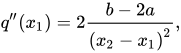
Setting t = 0 and t = 1 respectively in equations (5) and (6), one gets from (2) that indeed first derivatives q′(x₁) = k₁ and q′(x₂) = k₂, and also second derivatives

${\displaystyle q''(x_{1})=2{\frac {b-2a}{{(x_{2}-x_{1})}^{2}}},}$

7

${\displaystyle q''(x_{2})=2{\frac {a-2b}{{(x_{2}-x_{1})}^{2}}}.}$

8

If now (x_i, y_i), i = 0, 1, ..., n are n + 1 points, and

${\displaystyle q_{i}=(1-t)\,y_{i-1}+t\,y_{i}+t(1-t){\big (}(1-t)\,a_{i}+t\,b_{i}{\big )},}$

9

where i = 1, 2, ..., n, and ${\displaystyle t={\tfrac {x-x_{i-1}}{x_{i}-x_{i-1}}}}$ are n third-degree polynomials interpolating y in the interval x_i−1 ≤ x ≤ x_i for i = 1, ..., n such that q′_i (x_i) = q′_i+1(x_i) for i = 1, ..., n − 1, then the n polynomials together define a differentiable function in the interval x₀ ≤ x ≤ x_n, and

${\displaystyle a_{i}=k_{i-1}(x_{i}-x_{i-1})-(y_{i}-y_{i-1}),}$

10

${\displaystyle b_{i}=-k_{i}(x_{i}-x_{i-1})+(y_{i}-y_{i-1})}$

11

for i = 1, ..., n, where

${\displaystyle k_{0}=q_{1}'(x_{0}),}$

12

${\displaystyle k_{i}=q_{i}'(x_{i})=q_{i+1}'(x_{i}),\qquad i=1,\dots ,n-1,}$

13

${\displaystyle k_{n}=q_{n}'(x_{n}).}$

14

If the sequence k₀, k₁, ..., k_n is such that, in addition, q′′_i(x_i) = q′′_i+1(x_i) holds for i = 1, ..., n − 1, then the resulting function will even have a continuous second derivative.

From (7), (8), (10) and (11) follows that this is the case if and only if

${\displaystyle {\frac {k_{i-1}}{x_{i}-x_{i-1}}}+\left({\frac {1}{x_{i}-x_{i-1}}}+{\frac {1}{x_{i+1}-x_{i}}}\right)2k_{i}+{\frac {k_{i+1}}{x_{i+1}-x_{i}}}=3\left({\frac {y_{i}-y_{i-1}}{{(x_{i}-x_{i-1})}^{2}}}+{\frac {y_{i+1}-y_{i}}{{(x_{i+1}-x_{i})}^{2}}}\right)}$

15

for i = 1, ..., n − 1. The relations (15) are n − 1 linear equations for the n + 1 values k₀, k₁, ..., k_n.

For the elastic rulers being the model for the spline interpolation, one has that to the left of the left-most "knot" and to the right of the right-most "knot" the ruler can move freely and will therefore take the form of a straight line with q′′ = 0. As q′′ should be a continuous function of x, "natural splines" in addition to the n − 1 linear equations (15) should have

${\displaystyle q''_{1}(x_{0})=2{\frac {3(y_{1}-y_{0})-(k_{1}+2k_{0})(x_{1}-x_{0})}{{(x_{1}-x_{0})}^{2}}}=0,}$

${\displaystyle q''_{n}(x_{n})=-2{\frac {3(y_{n}-y_{n-1})-(2k_{n}+k_{n-1})(x_{n}-x_{n-1})}{{(x_{n}-x_{n-1})}^{2}}}=0,}$

i.e. that

${\displaystyle {\frac {2}{x_{1}-x_{0}}}k_{0}+{\frac {1}{x_{1}-x_{0}}}k_{1}=3{\frac {y_{1}-y_{0}}{(x_{1}-x_{0})^{2}}},}$

16

${\displaystyle {\frac {1}{x_{n}-x_{n-1}}}k_{n-1}+{\frac {2}{x_{n}-x_{n-1}}}k_{n}=3{\frac {y_{n}-y_{n-1}}{(x_{n}-x_{n-1})^{2}}}.}$

17

Eventually, (15) together with (16) and (17) constitute n + 1 linear equations that uniquely define the n + 1 parameters k₀, k₁, ..., k_n.

There exist other end conditions, "clamped spline", which specifies the slope at the ends of the spline, and the popular "not-a-knot spline", which requires that the third derivative is also continuous at the x₁ and x_n−1 points. For the "not-a-knot" spline, the additional equations will read:

${\displaystyle q'''_{1}(x_{1})=q'''_{2}(x_{1})\Rightarrow {\frac {1}{\Delta x_{1}^{2}}}k_{0}+\left({\frac {1}{\Delta x_{1}^{2}}}-{\frac {1}{\Delta x_{2}^{2}}}\right)k_{1}-{\frac {1}{\Delta x_{2}^{2}}}k_{2}=2\left({\frac {\Delta y_{1}}{\Delta x_{1}^{3}}}-{\frac {\Delta y_{2}}{\Delta x_{2}^{3}}}\right),}$

${\displaystyle q'''_{n-1}(x_{n-1})=q'''_{n}(x_{n-1})\Rightarrow {\frac {1}{\Delta x_{n-1}^{2}}}k_{n-2}+\left({\frac {1}{\Delta x_{n-1}^{2}}}-{\frac {1}{\Delta x_{n}^{2}}}\right)k_{n-1}-{\frac {1}{\Delta x_{n}^{2}}}k_{n}=2\left({\frac {\Delta y_{n-1}}{\Delta x_{n-1}^{3}}}-{\frac {\Delta y_{n}}{\Delta x_{n}^{3}}}\right),}$

where ${\displaystyle \Delta x_{i}=x_{i}-x_{i-1},\ \Delta y_{i}=y_{i}-y_{i-1}}$.

In case of three points the values for ${\displaystyle k_{0},k_{1},k_{2}}$ are found by solving the tridiagonal linear equation system

${\displaystyle {\begin{bmatrix}a_{11}&a_{12}&0\\a_{21}&a_{22}&a_{23}\\0&a_{32}&a_{33}\\\end{bmatrix}}{\begin{bmatrix}k_{0}\\k_{1}\\k_{2}\\\end{bmatrix}}={\begin{bmatrix}b_{1}\\b_{2}\\b_{3}\\\end{bmatrix}}}$

with

${\displaystyle a_{11}={\frac {2}{x_{1}-x_{0}}},}$

${\displaystyle a_{12}={\frac {1}{x_{1}-x_{0}}},}$

${\displaystyle a_{21}={\frac {1}{x_{1}-x_{0}}},}$

${\displaystyle a_{22}=2\left({\frac {1}{x_{1}-x_{0}}}+{\frac {1}{x_{2}-x_{1}}}\right),}$

${\displaystyle a_{23}={\frac {1}{x_{2}-x_{1}}},}$

${\displaystyle a_{32}={\frac {1}{x_{2}-x_{1}}},}$

${\displaystyle a_{33}={\frac {2}{x_{2}-x_{1}}},}$

${\displaystyle b_{1}=3{\frac {y_{1}-y_{0}}{(x_{1}-x_{0})^{2}}},}$

${\displaystyle b_{2}=3\left({\frac {y_{1}-y_{0}}{{(x_{1}-x_{0})}^{2}}}+{\frac {y_{2}-y_{1}}{{(x_{2}-x_{1})}^{2}}}\right),}$

${\displaystyle b_{3}=3{\frac {y_{2}-y_{1}}{(x_{2}-x_{1})^{2}}}.}$

For the three points

${\displaystyle (-1,0.5),\ (0,0),\ (3,3),}$

one gets that

${\displaystyle k_{0}=-0.6875,\ k_{1}=-0.1250,\ k_{2}=1.5625,}$

and from (10) and (11) that

${\displaystyle a_{1}=k_{0}(x_{1}-x_{0})-(y_{1}-y_{0})=-0.1875,}$

${\displaystyle b_{1}=-k_{1}(x_{1}-x_{0})+(y_{1}-y_{0})=-0.3750,}$

${\displaystyle a_{2}=k_{1}(x_{2}-x_{1})-(y_{2}-y_{1})=-3.3750,}$

${\displaystyle b_{2}=-k_{2}(x_{2}-x_{1})+(y_{2}-y_{1})=-1.6875.}$

In the figure, the spline function consisting of the two cubic polynomials ${\displaystyle q_{1}(x)}$ and ${\displaystyle q_{2}(x)}$ given by (9) is displayed.

• Akima spline
• Circular interpolation
• Cubic Hermite spline
• Centripetal Catmull–Rom spline
• Discrete spline interpolation
• Monotone cubic interpolation
• Non-uniform rational B-spline
• Multivariate interpolation
• Polynomial interpolation
• Smoothing spline
• Spline wavelet
• Thin plate spline
• Polyharmonic spline

• Schoenberg, Isaac J. (1946). "Contributions to the Problem of Approximation of Equidistant Data by Analytic Functions:Part A.—On the Problem of Smoothing or Graduation. A First Class of Analytic Approximation Formulae". Quarterly of Applied Mathematics. 4 (2): 45–99. doi:10.1090/qam/15914.
• Schoenberg, Isaac J. (1946). "Contributions to the Problem of Approximation of Equidistant Data by Analytic Functions:Part B.—On the Problem of Osculatory Interpolation. A Second Class of Analytic Approximation Formulae". Quarterly of Applied Mathematics. 4 (2): 112–141. doi:10.1090/qam/16705.

• Cubic Spline Interpolation Online Calculation and Visualization Tool (with JavaScript source code)
• "Spline interpolation", Encyclopedia of Mathematics, EMS Press, 2001 [1994]
• Dynamic cubic splines with JSXGraph
• Lectures on the theory and practice of spline interpolation
• Paper which explains step by step how cubic spline interpolation is done, but only for equidistant knots.
• Numerical Recipes in C, Go to Chapter 3 Section 3-3
• A note on cubic splines
• Information about spline interpolation (including code in Fortran 77)
• TinySpline:Open source C-library for splines which implements cubic spline interpolation
• SciPy Spline Interpolation:a Python package that implements interpolation
• Cubic Interpolation:Open source C#-library for cubic spline interpolation