Explore Black History

This article needs more citations. Please help improve this article by adding citations to reliable sources. Unsourced material may be challenged and removed. Find sources: "State variable" – news · newspapers · books · scholar · JSTOR (December 2009) (Learn how and when to remove this message)

A state variable is one of the set of mathematical variables that are used to describe the "state" of a system, e.g. of a dynamical system or a thermodynamical system.

Intuitively, the state of a system is the minimum amount of information about the system which is required to describe the present properties of the system (at least from a certain point of view within a modelling decision of defining a system and separating the system from its environment; if a family of systems is modelled, where the systems are distinguished by parameters, then these parameters are usually not considered to be state variables for the systems, but external system parameters. E.g. physical masses or physical coupling constants for describing interaction strength are given external system parameters, but not state variables for the system.)^[1]

In the mathematical model, bounded observables are often taken to be elements of an algebra of observables.^[2] Namely, if bounded observables, whose values might be added and multiplied, are modelled by using self-adjoint elements from a Cstar_algebra, then a state is a normalized positive element of the algebra's dual (a continuous linear functional ρ): If the system is in a state ${\textstyle \rho }$, then an observable ${\textstyle A}$ provides an observed value ${\textstyle \rho (A)=<\rho ,A>}$. (The brackets ${\textstyle <.,.>}$ denote the duality pairing between the dual space of the algebra and the algebra itself.) For example, if the observable is a function ${\textstyle f}$ from state space to real numbers, then evaluating the function at a point ${\textstyle x}$ provides a state ${\textstyle \rho _{x}}$ with ${\textstyle <\rho _{x},f>=f(x)}$, which is the point evaluation functional at point x. In this description, bounded state functions are certain bounded observables. It is possible to extend that notion to unbounded observables (examples in physics: a position component for full space, or a momentum component)^[3] for the general abstract case and therefore for more general unbounded state functions. Often, a maximal set of compatible commuting and independent observables can be chosen, and other compatible observables expressed as functions of these observables; then one has made a choice to express all compatible observables as functions of the independent observables, which become independent state variables.

For the definition and examples of states of a thermodynamic system see Thermodynamic state.

In thermodynamics, state variables are physically defined as large-scale characteristics or aggregate properties of a system which provide a macroscopic description of its states.^[4][5] In general, state variables have the following properties in common:

• They don't involve any special assumptions concerning the structure of matter, fields or radiation.
• They are few in number needed to describe the system.
• They are fundamental, as suggested by our sensory perceptions.
• They can be, in general, directly measured.^[4]

Classical algebras of observables are abelian^{[disambiguation needed]} (commutative), whereas algebras of quantum observables are Non-Abelian.^[6]

The macroscopic thermodynamic description of microscopic quantum systems is obtained as a Thermodynamic Limit of the microscopic system, and a corresponding algebra of observables is obtained, which allows for a definition of macroscopic observables. A distinction between abstract macroscopic observables and observables as thermodynamic state functions can be obtained as follows: For a specific macroscopic state, one uses the GNS-representation to obtain a representation of the algebra of observables as linear operators on a Hilbert space, one chooses a maximally Abelian algebra of compatible observables and applies the Gelfand transform for Abelian C*-algebras to represent abstract observables as functions on a representation space of states (Gelfand space). In general, such a description as functions on a Gelfand space depends on the macroscopic state chosen and is therefore representation dependent. State equations establish certain relations between these functions and therefore might define a variety of states as a set defined by equations for variables. Often, this variety is finite dimensional and then can be described by choosing certain observable state functions as independent state variables and express the other state functions as functions of these independent variables. In this sense, the independent state variables are used to parametrize the variety of states as functions from their domain to the variety of states, whereas general state functions are functions from the set of states to real (or complex) numbers. Composing these functions expresses the values of general observables as functions of the independent state variables, which makes them dependent state variables.

For instance, by describing a thermodynamic system by using the canonical ensemble of microscopic systems in the thermodynamic limit provides independent state variables ${\displaystyle T,V,N}$ (temperature, volume, particle number) corresponding to the formula ${\displaystyle dF=-SdT-pdV-\mu dN}$ for the thermodynamic free energy ${\displaystyle F=E-TS}$ with S = entropy, E = internal energy, μ = chemical potential. All other state variables can then be expressed as functions of T,V,N: For a monatomic ideal gas, the state equation for the pressure is the ideal gas law and pressure becomes a dependent state variable, the equation for entropy is the Sackur-Tetrode equation, internal energy can be obtained by requiring Joule's second law, and the chemical potential is computed via the Gibbs potential as described in the section Thermodynamic potentials of the article ideal gas.

All these variables depend only on the states, not on the history of how that state was obtained. This is an important property which makes them state variables, to be distinguished from e.g. process variables (better: process quantities), for which one cannot speak of attaining a particular value when the system is in a state. See the Non-Examples section below.

In the theory of Dynamical Systems, dynamical models that consist of coupled first-order differential equations are said to be in state-variable form.^[7]

• In mechanical systems, the position coordinates and velocities of mechanical parts are typical state variables; knowing these, it is possible to determine the future state of the objects in the system.
• In thermodynamics, a state variable is an independent variable of a state function. Examples include internal energy, enthalpy, temperature, entropy, chemical composition, pressure, volume, electric induction, magnetic induction. Heat and work are not state functions, but process functions.
• In electronic/electrical circuits, the voltages of the nodes and the currents through components in the circuit are usually the state variables. In any electrical circuit, the number of state variables are equal to the number of (independent) storage elements, which are inductors and capacitors. The state variable for an inductor is the current through the inductor, while that for a capacitor is the voltage across the capacitor.
• In ecosystem models, population sizes (or concentrations) of plants, animals and resources (nutrients, organic material) are typical state variables.

• In thermodynamics, heat is not a state variable. No system stores heat.^[8] One cannot speak of "the present amount of heat of a system". Heat is a process variable, which describes modes of transfer of energy when the system changes its state. Being a Process_function, heat depends on the process of how the system changes, not only on the system's state currently attained.
• In thermodynamics, mechanical or thermodynamic work is not a state variable. Work is another mode of transfer of energy when the system changes its state.

In control engineering and other areas of science and engineering, state variables are used to represent the states of a general system. The set of possible combinations of state variable values is called the state space of the system. The equations relating the current state of a system to its most recent input and past states are called the state equations, and the equations expressing the values of the output variables in terms of the state variables and inputs are called the output equations. As shown below, the state equations and output equations for a linear time invariant system can be expressed using coefficient matrices: A, B, C, and D

${\displaystyle A\in \mathbb {R} ^{N\times N},\quad B\in \mathbb {R} ^{N\times L},\quad C\in \mathbb {R} ^{M\times N},\quad D\in \mathbb {R} ^{M\times L},}$

where N, L and M are the dimensions of the vectors describing the state, input and output, respectively.

The state vector (vector of state variables) representing the current state of a discrete-time system (i.e. digital system) is ${\displaystyle x[n]}$, where n is the discrete point in time at which the system is being evaluated. The discrete-time state equations are

${\displaystyle x[n+1]=Ax[n]+Bu[n],}$

which describes the next state of the system (x[n+1]) with respect to current state and inputs u[n] of the system. The output equations are

${\displaystyle y[n]=Cx[n]+Du[n],}$

which describes the output y[n] with respect to current states and inputs u[n] to the system.

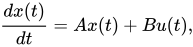
The state vector representing the current state of a continuous-time system (i.e. analog system) is ${\displaystyle x(t)}$, and the continuous-time state equations giving the evolution of the state vector are

${\displaystyle {\frac {dx(t)}{dt}}=Ax(t)+Bu(t),}$

which describes the continuous rate of change ${\textstyle {\frac {dx(t)}{dt}}}$ of the state of the system with respect to current state x(t) and inputs u(t) of the system. The output equations are

${\displaystyle y(t)=Cx(t)+Du(t),}$

which describes the output y(t) with respect to current states x(t) and inputs u(t) to the system.