Explore Black History

In econometrics and other applications of multivariate time series analysis, a variance decomposition or forecast error variance decomposition (FEVD) is used to aid in the interpretation of a vector autoregression (VAR) model once it has been fitted.^[1] The variance decomposition indicates the amount of information each variable contributes to the other variables in the autoregression. It determines how much of the forecast error variance of each of the variables can be explained by exogenous shocks to the other variables.

For the VAR (p) of form

${\displaystyle y_{t}=\nu +A_{1}y_{t-1}+\dots +A_{p}y_{t-p}+u_{t}}$ .

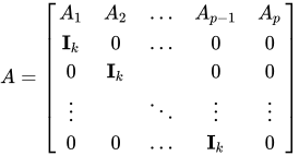
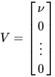
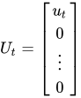
This can be changed to a VAR(1) structure by writing it in companion form (see general matrix notation of a VAR(p))

${\displaystyle Y_{t}=V+AY_{t-1}+U_{t}}$ where

${\displaystyle A={\begin{bmatrix}A_{1}&A_{2}&\dots &A_{p-1}&A_{p}\\\mathbf {I} _{k}&0&\dots &0&0\\0&\mathbf {I} _{k}&&0&0\\\vdots &&\ddots &\vdots &\vdots \\0&0&\dots &\mathbf {I} _{k}&0\\\end{bmatrix}}}$ , ${\displaystyle Y={\begin{bmatrix}y_{1}\\\vdots \\y_{p}\end{bmatrix}}}$, ${\displaystyle V={\begin{bmatrix}\nu \\0\\\vdots \\0\end{bmatrix}}}$ and ${\displaystyle U_{t}={\begin{bmatrix}u_{t}\\0\\\vdots \\0\end{bmatrix}}}$

where ${\displaystyle y_{t}}$, ${\displaystyle \nu }$ and ${\displaystyle u}$ are ${\displaystyle k}$ dimensional column vectors, ${\displaystyle A}$ is ${\displaystyle kp}$ by ${\displaystyle kp}$ dimensional matrix and ${\displaystyle Y}$, ${\displaystyle V}$ and ${\displaystyle U}$ are ${\displaystyle kp}$ dimensional column vectors.

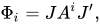
The mean squared error of the h-step forecast of variable ${\displaystyle j}$ is

${\displaystyle \mathbf {MSE} [y_{j,t}(h)]=\sum _{i=0}^{h-1}\sum _{l=1}^{k}(e_{j}'\Theta _{i}e_{l})^{2}={\bigg (}\sum _{i=0}^{h-1}\Theta _{i}\Theta _{i}'{\bigg )}_{jj}={\bigg (}\sum _{i=0}^{h-1}\Phi _{i}\Sigma _{u}\Phi _{i}'{\bigg )}_{jj},}$

and where

• ${\displaystyle e_{j}}$ is the j^th column of ${\displaystyle I_{k}}$ and the subscript ${\displaystyle jj}$ refers to that element of the matrix

• ${\displaystyle \Theta _{i}=\Phi _{i}P,}$ where ${\displaystyle P}$ is a lower triangular matrix obtained by a Cholesky decomposition of ${\displaystyle \Sigma _{u}}$ such that ${\displaystyle \Sigma _{u}=PP'}$, where ${\displaystyle \Sigma _{u}}$ is the covariance matrix of the errors ${\displaystyle u_{t}}$

• ${\displaystyle \Phi _{i}=JA^{i}J',}$ where ${\displaystyle J={\begin{bmatrix}\mathbf {I} _{k}&0&\dots &0\end{bmatrix}},}$ so that ${\displaystyle J}$ is a ${\displaystyle k}$ by ${\displaystyle kp}$ dimensional matrix.

The amount of forecast error variance of variable ${\displaystyle j}$ accounted for by exogenous shocks to variable ${\displaystyle l}$ is given by ${\displaystyle \omega _{jl,h},}$

${\displaystyle \omega _{jl,h}=\sum _{i=0}^{h-1}(e_{j}'\Theta _{i}e_{l})^{2}/MSE[y_{j,t}(h)].}$

This article needs more citations. Please help improve this article by adding citations to reliable sources. Unsourced material may be challenged and removed. Find sources: "Variance decomposition of forecast errors" – news · newspapers · books · scholar · JSTOR (March 2011) (Learn how and when to remove this message)

• Analysis of variance